2.3. PID digital controller: Python implementation

The aim of this tutorial is to implement temperature control on the TCLab board. The successive stages will be:

• definition of the continuous PID corrector from the transfer function identified previously.

• determining the maximum sampling time required to maintain a sufficient phase margin.

• digitalisation of the corrector in the form of a recurrence equation.

• analysis of real performances.

2.3.1. Requirements

Exercice: Complete the requirements for the temperature control in the following table.

Requirement	Assessment Criteria	Level
Control the temperature at 35°C	Temperature reference tracking	?
Settling time at 5 %	?
Overshoot	?
Disturbance rejection	?

2.3.2. Continuous controller

2.3.2.1. System transfer functions

In previous work, we identified the transfer function linking the heating control (input) \(Q_1\) to the temperature (output) \(T_1\) as second order:

\(G_1(p) = \frac{\Delta T_1(p)}{Q_1(p)}= \frac{0.65}{(27p + 1)(160p + 1)} \)

with \(\Delta T_1\) expressing the relative difference between the sensor temperature and the ambient temperature (around 20°C).

Question: Approximate the transfer function \(G_1(p)\) as a 1st order with pure delay.

2.3.2.2. Zielgler-Nichols method

The Ziegler-Nichols approach to setting PID controllers can be used as an initial parameterisation. This approach is based on a transfer function of the form: \( G(s) = \frac{Ke^{-Ls}}{\tau s + 1} \) with \(R=K/\tau\) with

• \(K\) : the steady-state gain;

• \(\tau\) : the dominant time-constant;

• \(L\) : the pure time-delay.

The form (P, PI, PD or PID) of the PID controller can then be chosen according to the value of \(\tau\) compared to \(L\) by using following table:

\(\frac{Time Constant}{Delay}=\frac{\tau}{L}\)	Best controller
\(\frac{\tau}{L} > 20 \)	On-Off controller
\(10 < \frac{\tau}{L} < 20 \)	P controller
\(5 < \frac{\tau}{L} < 10 \)	PI controller
\(2 < \frac{\tau}{L} < 5 \)	PID controller

Then the following table defines the parameters of a P, PI or PID controller: \(G_c(s)=k_p(1+\frac{1}{\tau_i s}+\tau_d s)=k_p+\frac{k_i}{s}+k_d s\)

Type	\(k_p\)	\(k_i\)	\(k_d\)
P	\(\frac{1}{RL}\)
PI	\(\frac{0.9}{RL}\)	\(\frac{3}{10RL^2}\)
PID	\(\frac{1.2}{RL}\)	\(\frac{0.6}{RL^2}\)	\(\frac{0.6}{R}\)

Exercice: Select and calculate the corrector.

%matplotlib inline

import numpy as np
import matplotlib.pyplot as plt

# Ziegler Nichols input parameter
tau = 160 # [s] time constant of the 1st order
L= 27 # [s] delay
K = 0.65 # [°/%] static gain

R=K/tau

# Controller type 
# ??

# controller coefficient with Ziegler Nichols approach

# ??


#print("PID coefficient (parrallel form): ")
#print("Kp = %.3f"%Kp)
#print("Ki = %.3f"%Ki)
#print("Kd = %.3f"%Kd)

2.3.2.3. Temporal performances

Exercice: Analyse the performance by simulation in terms of time: the following code should plot the time response \(T_1\) to a 1° step order. It is also interesting to plot the power demand \(Q_1\). You can use tf, step from control.matlab package.

import control.matlab as control

# system transfer function, based on second order model
G1 = 0.65*control.tf([1],[27,1])*control.tf([1],[160,1])

# controller and global model transfer functions

# ??

# Step response of the closed loop
t = np.linspace(0,400,1000)

# ??

#plt.plot(t,y, 'b', t,np.ones(1000),'g-')
#plt.xlabel('Time (s)')
#plt.ylabel('Output (t°C)')
#plt.show()

#plt.plot(t,Q, 'r')
#plt.xlabel('Time (s)')
#plt.ylabel('Power (%) input')
#plt.grid()
#plt.show()

2.3.2.4. Frequency performances

By plotting the Bode and Nichols diagrams in open or closed loops, we can establish the stability margins and the bandwidth.

Exercice: Analyse the frequency performances with Bode plots in open loop and closed loop. Adjust PID gains if necessary. Nichols diagram can be also usefull. You can use bode (with margins=True parameter), nichols from control.matlab package.

# Bode diagram of open loops

# Print phase and gain margins

# Print Nichols diagram

2.3.2.5. Optimal design of the controller

Exercice: Using the observations made, define an optimum design for the controller. This can be done using an optimisation algorithm such as scipy.optimize.fmin_slsqp(func, x0, bounds, f_ieqcons) from the scipy package where

• func is a function which return the objective to be minimised

• f_ieqcons is a function which return one or more constraints that must be positive in order to be respected.

• x0 is the initial set of parameter (vector) for objective anc ocnstraints functions.

import scipy

# Problem definition
def optim_model(x, param):
    Kp=x[0]
    Ki=x[1]
    Kd=0
    # controller and global model transfer functions
    # ??
    
    #if (param=='constraints'):
        # return [??]
    #elif (param=='objective'):
        # return ??

# Initial point
    
# InitPoint=np.array([??, ??])    

# bounds=[(min ?, max ?),
#        (min ?, max ?)]


# Resolution of the problem


contrainte = lambda x: optim_model(x, "constraints")
objectif = lambda x: optim_model(x, "objective")

# result = scipy.optimize.fmin_slsqp(func=objectif,x0=InitPoint, bounds=bounds, f_ieqcons=contrainte)

2.3.3. Digital controller

2.3.3.1. Definition of minimum sampling time

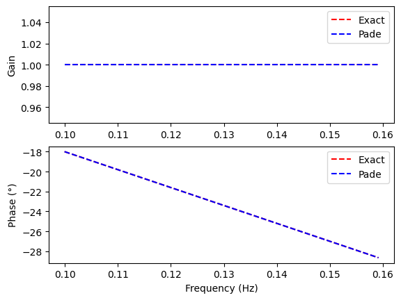
Exercise: Calculate the minimum sampling time required to avoid degrading the phase margin by more than 5°. Check your result using Padé’s approximation.

# Phase = -delay.w = 5° where delay=Ts/2
#gm, pm, wcg, wcp = control.margin(T)
# T_s = ??
T_s = 1 # To modify ?

print("Maximum sampling time: %.2e s"%T_s)

delay=T_s/2

num,den=control.pade(delay, 3)
pade=control.tf(num,den)

mag, phase, omega= control.bode(pade, plot=False, omega_limits=[1,2*3.14*.1], Hz=False)
                        

import matplotlib.pyplot as plt
import numpy as np

freq=omega/2/np.pi

plt.tight_layout()
fig, (ax1, ax2) = plt.subplots(2)    # get subplot axes

plt.sca(ax1)                 # magnitude plot
plt.plot(freq, [1]*len(omega),'r--', label='Exact')
plt.plot(freq, mag,'b--', label='Pade')
plt.ylabel('Gain')
plt.legend()

plt.sca(ax2)                 # phase plot
plt.plot(freq,-delay*omega*180/np.pi,'r--', label='Exact')
plt.plot(freq, phase*180/np.pi,'b--', label='Pade')
plt.xlabel('Frequency (Hz)')
plt.ylabel('Phase (°)')
plt.legend()

Maximum sampling time: 1.00e+00 s

<matplotlib.legend.Legend at 0x7f6d80ed7c70>

<Figure size 640x480 with 0 Axes>

#PIDSysPade=T*pade
#mag, phase, omega= control.bode(PIDSysPade, plot=True, Hz=True, initial_phase=0, margins=True)

2.3.4. Digital PID controller

2.3.4.1. Recurrence equation

Question: - Discretize the PID controller in the form of a recurrence equation.

Exercice: Define a PID function which returns
\(o_k = o_{k-1} + K_i e_k T_s + K_p (e_k-e_{k-1}) + \frac{K_d}{T_s}(e_k+ e_{k-2}-2e_{k-1})\)
where \(e_k\) is the error and \(o_k\) the output of the controller. The global keyword defines variables which belongs to the global scope.

def PID(order, measure):
    #global ??
    
    return max(0, min(100, o_k))

2.3.4.2. Real tests

The following cells can be used to test your controller. The first step is to check that your card is responding correctly.

%matplotlib inline
from tclab import TCLab

# if no card you can use the simulator:
# from tclab import TCLabModel as TCLab

from tclab import clock # from tclab import clock

# Start TCLab
# lab = TCLab()

tperiod = 20
tstep = 1

#lab.Q1(100)

#for t in clock(tperiod,tstep):
#    print("Time %4.1f sec. : Temp = %.2f"%(t,lab.T1))
           
#lab.Q1(0)

We will use a specific window to plot corrector results:
!pip install PySide6
!pip install PyQt6

import PyQt6
import PySide6

The following cell provides an initial implementation of PID control for heater T1.

print("Temperature 1: %0.2f °C"%(lab.T1))
print("Temperature 2: %0.2f °C"%(lab.T2))

import matplotlib.pyplot as plt
import numpy as np

time = []
Q1 = []
Kperror = []
T1 = []

Torder =35

tfinal = 400
tstep = T_s

%matplotlib qt

# Interactive mode
plt.ion()   # ion => interactive on / ioff => interactive off
plt.figure()
plt.plot(time, T1,'b-', label='T1')
plt.plot(time, Q1,'r-', label='Q1')
plt.plot(time, np.ones(len(time))*Torder,'g-', label='Order')
plt.xlabel('Time (s)')
plt.ylabel('Temperature (°C) - Heating power /2 (%)')
plt.legend()
plt.show(block=False)

for t in clock(tfinal, tstep):
    Tmes=lab.T1
    Q = PID(Torder, Tmes)
    lab.Q1(Q)
    time = time + [t]
    T1 = T1 + [Tmes]
    Q1 = Q1 + [Q]

    Title='T1 = %.1f °C - Q1 = %.1f'%(Tmes,Q)
    plt.title(Title)
    plt.plot(time, T1,'b-')
    plt.plot(time, Q1,'y-')
    plt.plot(time, np.ones(len(time))*Torder,'g-')
    #plt.show(block=False)
    plt.pause(0.05)

   
plt.ioff()    
print("\nTurn Heater Q1 Off")
lab.Q1(0)
#lab.close()

---------------------------------------------------------------------------
NameError                                 Traceback (most recent call last)
Cell In[13], line 1
----> 1 print("Temperature 1: %0.2f °C"%(lab.T1))
      2 print("Temperature 2: %0.2f °C"%(lab.T2))
      4 import matplotlib.pyplot as plt

NameError: name 'lab' is not defined

print("\nTurn Heater Q1 Off")
#lab.Q1(0)

Turn Heater Q1 Off

Finally, you can display the temperature and power curves:

%matplotlib inline

plt.ioff()  
plt.plot(time, T1,'b-', label='T1')
plt.plot(time, np.ones(len(time))*Torder,'g-', label='Order')
plt.xlabel('Time (s)')
plt.ylabel('Temperature (°C)')
plt.legend()
plt.show()

plt.plot(time, Q1,'r-', label='Q1')
plt.xlabel('Time (s)')
plt.ylabel('Puissance de chauffe (%)')
plt.legend()
plt.show()