6.4. Optimization of a motor/reducer set for a high dynamic application#
Written by Marc Budinger, INSA Toulouse, France
For applications wigh high bandwith mission profile and with high acceleration, the choice of a motor and a gearbox depends on a compromise function of the motor inertia and the reduction ratio.
Scipy and math packages will be used for this notebook in order to illustrate the optimization algorithms of python.
import scipy
import scipy.optimize
from math import pi
import timeit
6.4.1. Objectives and specifications#
The objective is to select the reduction ratio of a gear reducer in order to minimize the mass of the motor.
The application have to ensure :
a max force \(F_{load}\) of \(48 kN\) and a max acceleration of \(a_{max}=11.68 m/s²\)
a max speed \(v_{max}\) of 0.22 m/s
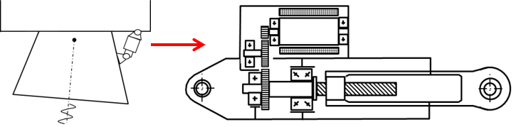
We will give here an example based on a linear actuator with a preselected roller screw (pitch of 10 mm/rev). We assume here, for simplification, the efficiency equal to 100%.
EMA components:
# Specifications
Max_speed=.22    # [m/s] max speed
Max_acceleration=11.68   # [m/s²] max acceleration (comined with max force)
Max_load=48000    # [N] max force

# Assumptions
Pitch=10e-3/2/pi  # [m/rad] roller screw pitch
6.4.2. Equations#
6.4.2.1. Sizing scenarios#
The brushless electric motor will be sized taking into account:
the maximum transient torque it must provide \(T_{max,app}\). This torque must take into account the acceleration of the motor’s inertia.
the maximum speed required for the application \(\Omega_{max,app}\).
Question: Provide the equations for maximum torque and maximum motor speed for the application requirements expressed above.
6.4.2.2. Parameter estimation with scaling laws#
Question: Show that the scaling laws used to express the characteristics of an electric motor can take the following forms:
\(M_{mot}=M_{ref}.\left(\frac{T_{max}}{T_{max,ref}}\right)^{3/3.5}\)
\(J_{mot}=J_{ref}.\left(\frac{T_{max}}{T_{max,ref}}\right)^{5/3.5}\)
\(\Omega_{max,motor}=\Omega_{ref}.\left(\frac{T_{max}}{T_{max,ref}}\right)^{-1/3.5}\)
where the reference values are: \(T_{max,ref}=13.4 N.m\), \(\Omega_{max,ref}=754 rad/s\), \(J_{ref}=2.9.10^{-4} kg.m^2\), \(M_{ref}=3.8 kg\).
6.4.3. Sizing code#
6.4.3.1. Design graph#
Exercice:
Represent the equations developed above in the form of an undirected graph.
Direct the graph by setting known values and solving various problems (subconstraints, overconstraints, algebraic loops).
Describe the optimization problem to be solved, detailing the optimization variables and their bounds, the calculations to be performed, the constraints to be satisfied, and the objective to be minimized.
6.4.3.2. Python code#
Exercice: Complete the following code cells to implement and solve an optimal sizing.
# Reference parameters for scaling laws
Tmax_ref=13.4    # [N.m]
Wmax_ref=754    # [rad/s]
Jref=2.9e-4/4     # [kg.m²]
Mref=3.8        # [kg]

# -----------------------
# sizing code
# -----------------------
# inputs:
# - param: optimisation variables vector (reduction ratio, oversizing coefficient)
# - arg: selection of output
# output:
# - objective if arg='Obj', problem characteristics if arg='Prt', constraints other else

# def SizingCode(param, arg):
#  Variables
    # ?? =param[0]
    # ?? =param[1]


# Objective and contraints
#    if arg=='Obj':
        ## return M
#    elif arg=='Prt':
#        print("* Optimisation variables:")
#        print("* Components characteristics:")
#        print("* Constraints (should be >0):")

#    else:
        ## return [,]
6.4.4. Optimization problem#
We will now use the opmization algorithms of the Scipy package to solve and optimize the configuration. We use here the SLQP algorithm without explicit expression of the gradient (Jacobian). A short course on Multidisplinary Gradient optimization algorithms and gradient optimization algorithm is given here:
Joaquim R. R. A. Martins (2012). A Short Course on Multidisciplinary Design Optimization. Univeristy of Michigan
The first step is to give an initial value of optimisation variables:
#Variables d'optimisation


# Vector of parameters
# parameters = scipy.array((??, ??))
We can print of the characterisitcs of the problem before optimization with the intitial vector of optimization variables:
# Initial characteristics before optimization
#print("-----------------------------------------------")
#print("Initial characteristics before optimization :")

#SizingCode(parameters, 'Prt')
#print("-----------------------------------------------")
Then we can solve the problem and print of the optimized solution:
# optimization with SLSQP algorithm
#contrainte=lambda x: SizingCode(x, 'Const')
#objectif=lambda x: SizingCode(x, 'Obj')
#result = scipy.optimize.fmin_slsqp(func=objectif, x0=parameters,
#                                   bounds=[(.1,10),(1,10)],
#                                   f_ieqcons=contrainte, iter=100, acc=1e-8)

# Final characteristics after optimization
#print("-----------------------------------------------")
#print("Final characteristics after optimization :")

#SizingCode(result, 'Prt')
#print("-----------------------------------------------")