IGBT estimation models with scaling laws [Student version]

9.2. IGBT estimation models with scaling laws [Student version]#

Written by Marc Budinger, INSA Toulouse, France

The estimation models calculate the component characteristics requested for their selection without requiring a detailed design. Scaling laws are particularly suitable for this purpose. This notebook illustrates the approach with IGBT component.

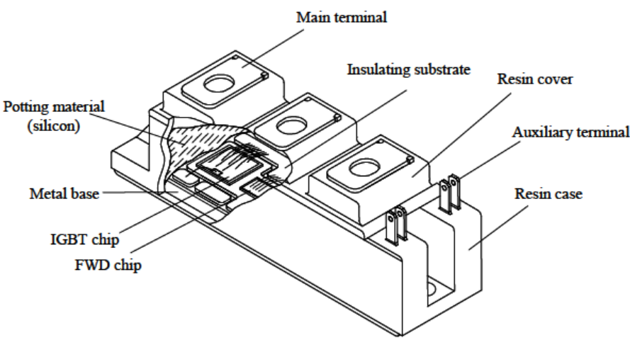
IGBT modules IGBTmodule

Validation of the obtained scaling laws is done thanks to linear regression on manufacturer datasheet.

The following article gives more details and other models for power converters:

Giraud, X., Budinger, M., Roboam, X., Piquet, H., Sartor, M., & Faucher, J. (2016). Optimal design of the Integrated Modular Power Electronics Cabinet. Aerospace Science and Technology, 48, 37-52.

9.2.1. Scaling law between Rth and I0#

9.2.1.1. Assumptions and notation#

The IGBT chip or MOSFET are constituted of many arranged structures called “unit cells”. The greater number the cells are, the lower the on-state voltage will be (parallel cells). The number of cells is assumed to be proportional to the current rating. We seek to establish the scaling laws for the same level of maximum voltage and the same technology. The thicknesses of the different layers (silicon, insulation, copper plate, …) will therefore be assumed to be constant.

Notation: The x* scaling ratio of a given parameter is calculated as \(x^*=\frac{x}{x_{ref}}\) where \(x_{ref}\) is the parameter taken as the reference and \(x\) the parameter under study.

Exercice 1 : propose a scaling law that links thermal resistance \(R_{th}\) to rated current \(I_0\). Estimate the thermal resistance for a 300 A component knowing the following reference component:
\(I_{0,ref} = 100 A\)
\(R_{th_JC,ref} = 0.27 °C/W\)

# Student Work

9.2.1.2. Validation with manufacturer datasheet#

We will compare the scaling law with a plot on manufacturer datasheet.

The first step is to import the data stored in a .csv file. We use for that functions from Panda package (with here an introduction to panda).

# Panda package Importation
import pandas as pd

# Read the .csv file with bearing data
path='https://raw.githubusercontent.com/SizingLab/sizing_course/main/laboratories/Lab-watt_project/assets/data/'
df = pd.read_csv(path+'DataIGBT.csv', sep=';')
# Print the head (first lines of the file)
df.head()

	REF	Emax	I0	Eon_off	Vcc_ref	Vf0	Rf0	Qrr	Rth_jc
0	SKMy50GB063D	600	50	4.3	300	0.9	15.0	3.2	0.50
1	SKMy50GB063D	600	75	5.5	300	0.9	13.3	3.7	0.35
2	SKMy50GB063D	600	100	7.0	300	0.9	10.0	6.0	0.27
3	SKMy50GB063D	600	200	18.5	300	0.9	5.5	12.7	0.14
4	SKMy50GB063D	600	300	27.0	300	0.9	3.7	18.0	0.09

We can now compare graphically the catalog data with scaling law:

blue points, catalog data
red line, scaling law
red point, the reference for scalin law.

For the plot, we use the matplotlib package.

import numpy as np
import matplotlib.pyplot as plt

# Add 1 mm diameter point
I0=np.linspace(10, 300, num=50)

# Scaling law
Rth=R_th_jc_ref*(I0/I0_ref)**(-1)

# plot
h, ax = plt.subplots(1,1,sharex=True)
ax.plot(I0, Rth, '--r',df['I0'],df['Rth_jc'],'.b', I0_ref, R_th_jc_ref, '.r')
ax.set_ylabel('Thermal resistance (junction to case) [°C/W]')
ax.set_xlabel('Rated current [A]')
ax.grid()

---------------------------------------------------------------------------
NameError                                 Traceback (most recent call last)
Cell In[3], line 8
      5 I0=np.linspace(10, 300, num=50)
      7 # Scaling law
----> 8 Rth=R_th_jc_ref*(I0/I0_ref)**(-1)
     10 # plot
     11 h, ax = plt.subplots(1,1,sharex=True)

NameError: name 'R_th_jc_ref' is not defined

9.2.2. Additional scaling laws#

The following table summarize the scaling laws which can be used for the sizing code.

9.2.2.1. IGBT#

	Scaling laws	References
Definition parameter :
Current	\(I\)	\(80 A\)
Maximum voltage	\(U_{max}^* = 1\)	\(900 V\)
Voltage drop	\(U_0^*=1\)	\(1 V\)
Dynamic resistance	\(R_0^=I^{-1}\)	20 m\({\Omega}\)
Commutation losses	\((E_{on}+E_{off})^=I^ U^*\)	\(8.2 mJ\) for \(U=450 V\)
Thermal resistance	\(R_{th_JC}^=I^{-1}\)	\(0.30 °C/W\)

9.2.2.2. Diode (current evolution equal to IGBT current)#

	Scaling laws	References
Definition parameter :
Current	\(I\)	\(41 A\)
Maximum voltage	\(U_{max}^* = 1\)	\(900 V\)
Voltage drop	\(U_0^*=1\)	\(1 V\)
Dynamic resistance	\(R_0^=I^{-1}\)	\(15 m\Omega\)
Commutation losses	\(t_{rr}I_{RM}^{}=I^U^*\)	\(17.2 mJ\) for \(E=600 V\)
Thermal resistance	\(R_{th_JC}^{}=I^{-1}\)	\(0.47 °C/W\)

Exercice 2: Calculate the characteristics (electric/thermal resistances and commutation losses) of a 10A IGBT/DIODE operating under a 300V DC bus.

# Student work