
9.3. TP1 - Case study specification [Student Version]#
Written by Marc Budinger, INSA Toulouse, France
The objective of this notebook is to develop tools to:
generate typical point-ot-point mission profiles to analyse the energetic performance of different mobility;
optimize thoose given profiles shapes/strategy to minimize consumption;
In order to have flexibility in the definition of the case studies, an object-oriented programming approach will be used and links will be given to understand the formalism.
9.3.1. Table of Contents#
9.3.2. Vehicles definition#
Different types of urban electric vehicles exist (tram, trolley bus, electric bus), we can define a general vehicle class which can represent the multiple possible supports.
class vehicle:
    def __init__(self, MaxSpeed, MaxAcc, NumberPass, Weight, Crr, Cd, FrontArea):
        self.MaxSpeed = MaxSpeed # [m/s] maximal speed
        self.NumberPass = NumberPass # [-] passenger capacity (pass/veh)
        self.Weight = Weight # [kg] effective weight (with passenger: add 62kg/pass)
        self.Crr = Crr # [-] rolling resistance coefficient
        self.Cd = Cd # [-] drag coefficient
        self.FrontArea = FrontArea # [m²] frontal area
        self.update_acc(MaxAcc)

    def update_acc(self, MaxAcc):
        self.MaxAcc = MaxAcc # [m/s²] maximal acceleration
        self.Fmax = self.Weight*MaxAcc # [N] max traction force
        self.Pmax = self.Fmax*self.MaxSpeed # [W] max corner power
Here you will find some useful vehicle characteristics for the rest of the study.
Attribute |
Tram |
Trolleybus |
Bus |
Car (Tesla 3) |
|---|---|---|---|---|
Maximum operational speed |
60 km/h |
60 km/h |
50 km/h |
100 km/h (1st gear) |
Acceleration and braking |
1.2 m/s² |
1.2 m/s² |
1.2 m/s² |
4.6 m/s² |
Passenger capacity |
220 |
138 |
95 |
4 |
Vehicle effective weight @ 62 kg/p |
57049 kg |
27656 kg |
19500 kg |
1800 kg |
Rolling resistance coefficient |
0.006 |
0.015 |
0.015 |
0.015 |
Aerodynamic drag coefficient |
0.6 |
0.6 |
0.6 |
0.23 |
Frontal area |
8.5 m² |
8.5 m² |
8.5 m² |
2.22 m² |
Exercise 1: Define the 4 instances corresponding to the vehicles described in the above table.
Tram = vehicle(MaxSpeed=60*1e3/3600, MaxAcc=1.2, NumberPass=220, Weight=57049, Crr=0.006, Cd=0.6, FrontArea=8.5)
9.3.3. Mission profile definition and consumption simulation#
The objective now is to simulate the dynamic evolution of the main mechanical quantities (position, speed, acceleration, traction/braking force, traction/braking power and cumulated energy) on typical sections of urban routes (a point-to-point scenario).
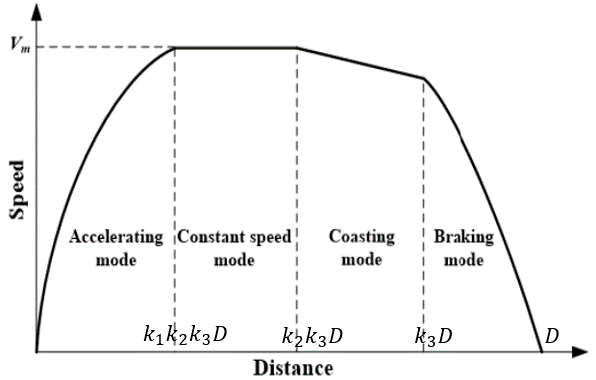
When a vehicle travels from point A (Starting point - v=0km/h) to point B (Stopping point - v=0km/h) it generally passes through four stages namely:
Acceleration portion (traction force is considered constant);
Maintained speed portion (or null acceleration);
Coasting/freewheel portion: traction/braking force is null;
Braking portion (braking force is considered constant).
The control points for switching from one portion to the other one are defined in the following code by using 3 ratio parameters \(k_1, k_2, k_3\) as shown in the figure below:
Exercise 2: Try to find the shape of the acceleration=f(distance) and propulsive\braking-force=f(distance) curves.
A code skeleton initial implementation is given to define a point-to-point dynamic simulation. The idea is to propose a simple Euler inegration of vehicle longitudinal dynamics and calculate associated data (power, energy) across the entire profile.
Exercise 3: Based on available data, implement longitudinal dynamic differential equation (PFD) in CODE 2 section. What force/parameter evolution could be added to take into account variations in altitude?
import numpy as np
import matplotlib.pyplot as plt

class SimulSection:

    def __init__(self, Vehicle, Distance, MeanSpeed, BrakeRatioMax, dt):

        # Parameters definition
        self.Vehicle = Vehicle # store vehicle class instance
        self.Distance = Distance # [m] A-B distance to travel
        self.MeanSpeed = MeanSpeed # [m/s] Mean Speed
        self.TravelTime = self.Distance / self.MeanSpeed  # [s] Travel time
        self.BrakeRatioMax = BrakeRatioMax # [-], <1 =F_braking/f_propulsion (to reproduce driver behavior)
        self.dt = dt # Time step for numerical solver

        # Constants
        self.rho = 1.25 # [kg/m3] air density
        self.g = 9.81 # [m/s²] gravity

        # Validate vehicle limits match specifications (print warning):
        #    - max acceleration/braking vs. Vmean and distance (triangular acceleration profile)
        #    - Vmean vs. max speed on trapezoidal profile
        ###############################################
        # CODE 1
        ###############################################

    def update_acc(self, MaxAcc):
        self.Vehicle.update_acc(MaxAcc)
        # Validate vehicle limits match specifications (print warning):
        #    - max acceleration/braking vs. Vmean and distance (triangular acceleration profile)
        #    - Vmean vs. max speed on trapezoidal profile
        ###############################################
        # CODE 1
        ###############################################

    # local derivative of the vehicle state vector y (y=[x, dx/dt], x being the longitudinal position)
    def derivative(self, y, F):

        # state
        x, dxdt = y

        # Define derivative d²xdt²
        ###############################################
        # CODE 2
        ###############################################

        dydt = [dxdt, dxdt2]
        return dydt


    # https://perso.crans.org/besson/publis/notebooks/Runge-Kutta_methods_for_ODE_integration_in_Python.html
    # solver numerique

    def solver(self, profile_ratios):

        # save profile ratios
        k1, k2, k3 = profile_ratios
        dt=self.dt # [s] integration time step

        # initialise vectors (time, position, speed, acceleration, power @ wheel, force @ wheel, energy @ wheel)
        self.tsection = [0]
        self.xsection = [0]
        self.vsection = [0]
        self.asection = [0]
        self.psection = [0]
        self.Fsection = [0]
        self.NRJsection = [0]

        # while vehicle speed remains positive point B is not reached
        y= np.array([0, 0])
        while (y[1]>=0):

            # Depending on profile section/portion, define wheel force
            if (y[0]<k1*k2*k3*self.Distance):
                F=self.Vehicle.Fmax
            elif (y[0]<k3*k2*self.Distance):
                F=(self.Vehicle.Crr*self.Vehicle.Weight*self.g+1/2*self.rho*self.Vehicle.FrontArea*self.Vehicle.Cd*y[1]**2)*np.sign(y[1])
            elif (y[0]<k3*self.Distance):
                F=0
            else:
                F=-self.BrakeRatioMax*self.Vehicle.Fmax

            # Perform a simple Euler integration from t to t+dt
            dydt = self.derivative(y, F)
            y = y + dt*np.array(dydt)

            # Save vectors
            self.tsection = self.tsection + [self.tsection[-1]+dt]
            self.xsection = self.xsection + [y[0]]
            self.vsection = self.vsection + [y[1]]
            self.psection = self.psection + [y[1]*F]
            self.asection = self.asection + [dydt[1]]
            self.Fsection = self.Fsection + [F]
            self.NRJsection = self.NRJsection + [self.NRJsection[-1]+y[1]*F*dt]

    # Plot all the results vs. specification in graphs
    def plot(self):
        fig, axs = plt.subplots(3,2)

        axs[0,0].plot(self.tsection,self.xsection,'b-',label='Simulation')
        axs[0,0].plot(self.tsection,self.Distance*np.ones(len(self.tsection)),'g-',label='Specified distance')
        axs[0,0].set_ylabel("Position (m)")
        axs[0,0].set_xlabel('Time (s)')
        axs[0,0].legend()
        axs[0,0].grid()

        axs[1,0].plot(self.tsection, self.vsection,'b-', label='Simulation')
        axs[1,0].plot(self.tsection, self.MeanSpeed*np.ones(len(self.tsection)),'g-',label='Specified mean speed')
        axs[1,0].plot(self.tsection, np.mean(self.vsection)*np.ones(len(self.tsection)),'r--',label='Profile mean speed')
        axs[1,0].set_ylabel("Speed (m/s)")
        axs[1,0].set_xlabel('Time (s)')
        axs[1,0].legend()
        axs[1,0].grid()

        axs[0,1].plot(self.tsection, self.Fsection,'b-')
        axs[0,1].set_ylabel("Force (N)")
        axs[0,1].set_xlabel('Time (s)')
        axs[0,1].grid()

        axs[2,0].plot(self.tsection, self.asection,'b-')
        axs[2,0].set_ylabel("Acceleration (m/s²)")
        axs[2,0].set_xlabel('Time (s)')
        axs[2,0].grid()

        axs[1,1].plot(self.tsection, np.array(self.psection)*1e-3,'b-')
        axs[1,1].set_ylabel("Power (kW)")
        axs[1,1].set_xlabel('Time (s)')
        axs[1,1].grid()

        axs[2,1].plot(self.tsection, np.array(self.NRJsection)*1e-3,'b-')
        axs[2,1].set_ylabel("Energy (kJ)")
        axs[2,1].set_xlabel('Time (s)')
        axs[2,1].grid()

        fig.tight_layout()

    def ConsumptionPerPax(self,x):
        self.solver(x)
        print("Consumption per passenger: %.2f kJ/(Pax.km)"%(self.NRJsection[-1]/self.Vehicle.NumberPass/self.Distance))
        return (self.NRJsection[-1]/self.Vehicle.NumberPass/self.Distance)

    def MaxEnergyPoint(self,x):
        self.solver(x)
        print("Max energy discharge: %.0f kJ"%(max(self.NRJsection)*1e-3))
        return max(self.NRJsection)*1e-3

    def MaxPowerPoints(self,x):
        self.solver(x)
        print("Max power discharge: %.0f kW"%(max(self.psection)*1e-3))
        print("Max power recharge: %.0f kW"%(min(self.psection)*1e-3))
        return max(self.psection)*1e-3, min(self.psection)*1e-3
To check that the developed code does not containt errors, let us apply following Tram example:
# Definition of the section under study
Travel_Tram = SimulSection(Vehicle=Tram, Distance=670, MeanSpeed=26*1e3/3600, BrakeRatioMax=1.0, dt=1.0)
print('Duration of traject for given mean speed: {:.2f}s'.format(670/(26*1e3/3600)))

# Profile integration, plotting and consummption per passenger evaluation
X=[0.036125972011676784, 1, 0.9638740279883232]
Travel_Tram.solver(X)
Travel_Tram.plot()
Travel_Tram.ConsumptionPerPax(X)
Travel_Tram.MaxEnergyPoint(X)
Travel_Tram.MaxPowerPoints(X)
Duration of traject for given mean speed: 92.77s
---------------------------------------------------------------------------
NameError                                 Traceback (most recent call last)
Cell In[4], line 7
      5 # Profile integration, plotting and consummption per passenger evaluation
      6 X=[0.036125972011676784, 1, 0.9638740279883232]
----> 7 Travel_Tram.solver(X)
      8 Travel_Tram.plot()
      9 Travel_Tram.ConsumptionPerPax(X)

Cell In[3], line 84, in SimulSection.solver(self, profile_ratios)
     81     F=-self.BrakeRatioMax*self.Vehicle.Fmax
     83 # Perform a simple Euler integration from t to t+dt
---> 84 dydt = self.derivative(y, F)
     85 y = y + dt*np.array(dydt)
     87 # Save vectors

Cell In[3], line 47, in SimulSection.derivative(self, y, F)
     40 x, dxdt = y
     42 # Define derivative d²xdt²
     43 ###############################################
     44 # CODE 2
     45 ###############################################
---> 47 dydt = [dxdt, dxdt2]
     48 return dydt

NameError: name 'dxdt2' is not defined
When we look at the speed profile we can easily imagine two extrema cases :
a triangular speed profile (acceleration/deceleration, without constant speed & freewheel portion)
a trapezoidal speed profile (without freewheel portion) They kind of relate to maximum performances achievable given the vehicle parameters. The idea here is to compare the profile defined by user (average speed/distance, maximum brake decceleration) to extreme vehicle performances to see if it is feasible (i.e. a [k1, k2, k3] can be found).
Exercise 4: Give the relationship between acceleration, braking ratio, average speed and distance traveled for triangular speed profile (k1=k2=1) if we assume the acceleration and braking phases are perfectly linear (i.e. resistive force negligible)! Start first to link k3 to braking ratio
Exercise 5: Give the relationship between k1 and k3 (k2=1) if we assume the acceleration and braking phases are perfectly linear (the resistive force is neglected) and equal (braking ratio =1 to simplify). Find then the relationship between max speed, average speed, ditance and acceleration. Then highligh the link between k3, max speed, acceleration and distance.
Exercise 6: Complete CODE 1 section with checks and warnings based on exercice 4 calculations (compare also max speed to vehicle max speed). Check warning using following low acceleration tram instance.
import copy

# Test of lower acceleration
Travel_Tram_low_acc = copy.deepcopy(Travel_Tram)
Travel_Tram_low_acc.update_acc(0.3)
print("")

# Test of lower max speed
Travel_Tram_low_acc.Vehicle.MaxSpeed = 30*1e3/3600
Travel_Tram_low_acc.update_acc(0.5)
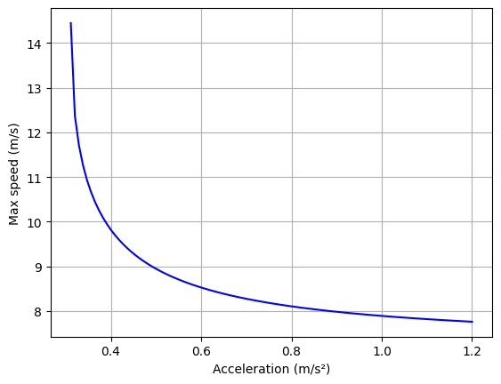
We whant to plot the curve linking the reached maximum speed and the maximum acceleration for a trapezoidal profile. Check that following formulation match your previous equation solution.
# Evalutation of maximum speed and k1/k3 coefficients
from scipy.optimize import root
a=np.linspace(4*Travel_Tram.MeanSpeed**2/Travel_Tram.Distance, Tram.MaxAcc, 100)
vmax = a/2*(Travel_Tram.Distance/Travel_Tram.MeanSpeed-((Travel_Tram.Distance/Travel_Tram.MeanSpeed)**2-4*Travel_Tram.Distance/a)**0.5)
plt.plot(a,vmax,'b-')
plt.xlabel('Acceleration (m/s²)')
plt.ylabel('Max speed (m/s)')
plt.grid()
plt.show()
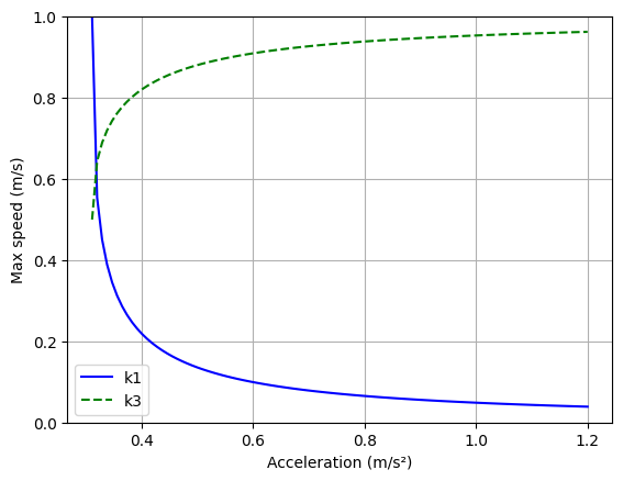
k3 = 1-vmax**2/(2*a*Travel_Tram.Distance)
k1 = (1-k3)/k3
plt.plot(a,k1,'b-',label='k1')
plt.plot(a,k3,'g--',label='k3')
plt.xlabel('Acceleration (m/s²)')
plt.ylabel('Max speed (m/s)')
plt.grid()
plt.legend()
plt.ylim([0, 1])
plt.show()
Exercise 7: Let us evaluate the Tram performance for different maximum accelerations a=[0.5, 0.8, 1.1] to see a trend on energy demand. As whe did not put any efficiency and by comparing the different resistive forces (Crr=0.006/10, so lowered to a factor 10) can this result be explained?
from numpy import interp

Travel_Tram.BrakeRatioMax=1.0
Travel_Tram.dt=0.1

# Treat 0.5m/s² acceleration
k1_value = interp(0.5, a, k1)
k3_value = interp(0.5, a, k3)
Travel_Tram.update_acc(0.5)
X = [k1_value, 1, k3_value]
Travel_Tram.solver(X)
Travel_Tram.plot()
Travel_Tram.MaxEnergyPoint(X)

# Treat 0.8m/s² acceleration
k1_value = interp(0.8, a, k1)
k3_value = interp(0.8, a, k3)
Travel_Tram.update_acc(0.8)
X = [k1_value, 1, k3_value]
Travel_Tram.solver(X)
Travel_Tram.plot()
Travel_Tram.MaxEnergyPoint(X)

# Treat 1.1m/s² acceleration
k1_value = interp(1.1, a, k1)
k3_value = interp(1.1, a, k3)
Travel_Tram.update_acc(1.1)
X = [k1_value, 1, k3_value]
Travel_Tram.solver(X)
Travel_Tram.plot()
Travel_Tram.MaxEnergyPoint(X)
---------------------------------------------------------------------------
NameError                                 Traceback (most recent call last)
Cell In[7], line 11
      9 Travel_Tram.update_acc(0.5)
     10 X = [k1_value, 1, k3_value]
---> 11 Travel_Tram.solver(X)
     12 Travel_Tram.plot()
     13 Travel_Tram.MaxEnergyPoint(X)

Cell In[3], line 84, in SimulSection.solver(self, profile_ratios)
     81     F=-self.BrakeRatioMax*self.Vehicle.Fmax
     83 # Perform a simple Euler integration from t to t+dt
---> 84 dydt = self.derivative(y, F)
     85 y = y + dt*np.array(dydt)
     87 # Save vectors

Cell In[3], line 47, in SimulSection.derivative(self, y, F)
     40 x, dxdt = y
     42 # Define derivative d²xdt²
     43 ###############################################
     44 # CODE 2
     45 ###############################################
---> 47 dydt = [dxdt, dxdt2]
     48 return dydt

NameError: name 'dxdt2' is not defined
9.3.4. Automatically find speed profile decomposition (k1, k2, k3) with an optimization process#
In a more general case and contrary to the previous hypothesis, the braking decceleration is not necessarily egual in magnitude to the acceleration, especially when doing regenerative braking (maximum power limited by energy storage). The following paper shows that it is possible to optimize the consumption of a tram by optimizing its profile:
Tian, Z., Zhao, N., Hillmansen, S., Roberts, C., Dowens, T., & Kerr, C. (2019). SmartDrive: Traction energy optimization and applications in rail systems. IEEE Transactions on Intelligent Transportation Systems, 20(7), 2764-2773.
The previous class is extended to allow optimizing the parameters defining the profile shape \(k_1, k_2, k_3\) with respect to different objectives: energy consumption (considering regenerative power) and max energy discharge. Only the first objective is given.
Exercise 8: Write the gradient optimization for max energy discharge objective (modify directely the code and use arguments of objectifConco method).
from scipy.optimize import fmin_slsqp, differential_evolution
import numpy

class OptimSection(SimulSection):

    # Define objective to optimize: here normalized (divided by rolling resistance equivalent work) total consummed energy (including regenerative power)
    def objectifConso(self, x, *args):
        self.solver(x)
        NRJmin = self.xsection[-1]*self.Vehicle.Weight*self.g*self.Vehicle.Crr
        if args[0]:
            pen=numpy.sum(-1e2*numpy.array(self.contraintes(x)))
            pen=pen*(pen>0)
        else:
            pen=0.0
        return ((self.NRJsection[-1]*(args[2]==1)+max(self.NRJsection)*(args[2]==2))/NRJmin+pen)

    # Define constraints to verify: traveled distance, traveled time (similar to average speed)
    def contraintes(self, x, *args):
        self.solver(x)
        TimeTravel = self.Distance / self.MeanSpeed
        return [(self.xsection[-1]-self.Distance)/self.Distance, (TimeTravel-self.tsection[-1])/TimeTravel]

    # SLSQP gradient optimization with constraints
    def optimizeConso_gradient(self, x0):
        Xbound= [(0.0, 0.3), (0.1, 1), (0.5,.99)]
        Xopt=fmin_slsqp(func=self.objectifConso, x0=x0, f_ieqcons = self.contraintes, bounds=Xbound, args=[False, 'gradient', 1], epsilon=1e-2)
        return Xopt

    # Differential evolution optimization
    def optimizeConso_genetic(self, x0):
        Xbound= [(0.0, 0.3), (0.1, 1), (0.5,0.99)]
        res=differential_evolution(func=self.objectifConso, x0=x0, args=[True, 'genetic', 1], bounds=Xbound)
        print(res)
        return res.x
The usage of the class is quite simular that the previous one, but it adds an optimizeConso method which enables us to find the \(k_1, k_2, k_3\) set. Let us apply it to the tram travel.
# Definition of the section under study
Travel_optim = OptimSection(Vehicle=Tram, Distance=670, MeanSpeed=26*1e3/3600, BrakeRatioMax=1.0, dt=1.0)

# Initial variables vector
X_init=[0.05, 0.6, 0.98]

# Optimization of the consumption with gradient
Xopt1=Travel_optim.optimizeConso_gradient(X_init)
print("Optimal vector :", Xopt1)
print("Constraints vector :", Travel_optim.contraintes(Xopt1))

Travel_optim.solver(Xopt1)
Travel_optim.plot()
Travel_optim.ConsumptionPerPax(Xopt1)
Travel_optim.MaxEnergyPoint(Xopt1)
---------------------------------------------------------------------------
NameError                                 Traceback (most recent call last)
Cell In[9], line 8
      5 X_init=[0.05, 0.6, 0.98]
      7 # Optimization of the consumption with gradient
----> 8 Xopt1=Travel_optim.optimizeConso_gradient(X_init)
      9 print("Optimal vector :", Xopt1)
     10 print("Constraints vector :", Travel_optim.contraintes(Xopt1))

Cell In[8], line 26, in OptimSection.optimizeConso_gradient(self, x0)
     24 def optimizeConso_gradient(self, x0):
     25     Xbound= [(0.0, 0.3), (0.1, 1), (0.5,.99)]
---> 26     Xopt=fmin_slsqp(func=self.objectifConso, x0=x0, f_ieqcons = self.contraintes, bounds=Xbound, args=[False, 'gradient', 1], epsilon=1e-2)
     27     return Xopt

File /opt/hostedtoolcache/Python/3.9.25/x64/lib/python3.9/site-packages/scipy/optimize/_slsqp_py.py:210, in fmin_slsqp(func, x0, eqcons, f_eqcons, ieqcons, f_ieqcons, bounds, fprime, fprime_eqcons, fprime_ieqcons, args, iter, acc, iprint, disp, full_output, epsilon, callback)
    206 if f_ieqcons:
    207     cons += ({'type': 'ineq', 'fun': f_ieqcons, 'jac': fprime_ieqcons,
    208               'args': args}, )
--> 210 res = _minimize_slsqp(func, x0, args, jac=fprime, bounds=bounds,
    211                       constraints=cons, **opts)
    212 if full_output:
    213     return res['x'], res['fun'], res['nit'], res['status'], res['message']

File /opt/hostedtoolcache/Python/3.9.25/x64/lib/python3.9/site-packages/scipy/optimize/_slsqp_py.py:338, in _minimize_slsqp(func, x0, args, jac, bounds, constraints, maxiter, ftol, iprint, disp, eps, callback, finite_diff_rel_step, **unknown_options)
    334 # Set the parameters that SLSQP will need
    335 # meq, mieq: number of equality and inequality constraints
    336 meq = sum(map(len, [atleast_1d(c['fun'](x, *c['args']))
    337           for c in cons['eq']]))
--> 338 mieq = sum(map(len, [atleast_1d(c['fun'](x, *c['args']))
    339            for c in cons['ineq']]))
    340 # m = The total number of constraints
    341 m = meq + mieq

File /opt/hostedtoolcache/Python/3.9.25/x64/lib/python3.9/site-packages/scipy/optimize/_slsqp_py.py:338, in <listcomp>(.0)
    334 # Set the parameters that SLSQP will need
    335 # meq, mieq: number of equality and inequality constraints
    336 meq = sum(map(len, [atleast_1d(c['fun'](x, *c['args']))
    337           for c in cons['eq']]))
--> 338 mieq = sum(map(len, [atleast_1d(c['fun'](x, *c['args']))
    339            for c in cons['ineq']]))
    340 # m = The total number of constraints
    341 m = meq + mieq

Cell In[8], line 19, in OptimSection.contraintes(self, x, *args)
     18 def contraintes(self, x, *args):
---> 19     self.solver(x)
     20     TimeTravel = self.Distance / self.MeanSpeed
     21     return [(self.xsection[-1]-self.Distance)/self.Distance, (TimeTravel-self.tsection[-1])/TimeTravel]

Cell In[3], line 84, in SimulSection.solver(self, profile_ratios)
     81     F=-self.BrakeRatioMax*self.Vehicle.Fmax
     83 # Perform a simple Euler integration from t to t+dt
---> 84 dydt = self.derivative(y, F)
     85 y = y + dt*np.array(dydt)
     87 # Save vectors

Cell In[3], line 47, in SimulSection.derivative(self, y, F)
     40 x, dxdt = y
     42 # Define derivative d²xdt²
     43 ###############################################
     44 # CODE 2
     45 ###############################################
---> 47 dydt = [dxdt, dxdt2]
     48 return dydt

NameError: name 'dxdt2' is not defined
# Optimization of the consumption with genetic algorithm
X_init=[0.3, 1.0, 0.95]
Xopt1=Travel_optim.optimizeConso_genetic(X_init)
print("Optimal vector :", Xopt1)
print("Constraints vector :", Travel_optim.contraintes(Xopt1))

Travel_optim.solver(Xopt1)
Travel_optim.plot()
Travel_optim.ConsumptionPerPax(Xopt1)
Travel_optim.MaxEnergyPoint(Xopt1)
---------------------------------------------------------------------------
NameError                                 Traceback (most recent call last)
Cell In[10], line 3
      1 # Optimization of the consumption with genetic algorithm
      2 X_init=[0.3, 1.0, 0.95]
----> 3 Xopt1=Travel_optim.optimizeConso_genetic(X_init)
      4 print("Optimal vector :", Xopt1)
      5 print("Constraints vector :", Travel_optim.contraintes(Xopt1))

Cell In[8], line 32, in OptimSection.optimizeConso_genetic(self, x0)
     30 def optimizeConso_genetic(self, x0):
     31     Xbound= [(0.0, 0.3), (0.1, 1), (0.5,0.99)]
---> 32     res=differential_evolution(func=self.objectifConso, x0=x0, args=[True, 'genetic', 1], bounds=Xbound)
     33     print(res)
     34     return res.x

File /opt/hostedtoolcache/Python/3.9.25/x64/lib/python3.9/site-packages/scipy/optimize/_differentialevolution.py:502, in differential_evolution(func, bounds, args, strategy, maxiter, popsize, tol, mutation, recombination, seed, callback, disp, polish, init, atol, updating, workers, constraints, x0, integrality, vectorized)
    485 # using a context manager means that any created Pool objects are
    486 # cleared up.
    487 with DifferentialEvolutionSolver(func, bounds, args=args,
    488                                  strategy=strategy,
    489                                  maxiter=maxiter,
   (...)
    500                                  integrality=integrality,
    501                                  vectorized=vectorized) as solver:
--> 502     ret = solver.solve()
    504 return ret

File /opt/hostedtoolcache/Python/3.9.25/x64/lib/python3.9/site-packages/scipy/optimize/_differentialevolution.py:1155, in DifferentialEvolutionSolver.solve(self)
   1150     self.feasible, self.constraint_violation = (
   1151         self._calculate_population_feasibilities(self.population))
   1153     # only work out population energies for feasible solutions
   1154     self.population_energies[self.feasible] = (
-> 1155         self._calculate_population_energies(
   1156             self.population[self.feasible]))
   1158     self._promote_lowest_energy()
   1160 # do the optimization.

File /opt/hostedtoolcache/Python/3.9.25/x64/lib/python3.9/site-packages/scipy/optimize/_differentialevolution.py:1315, in DifferentialEvolutionSolver._calculate_population_energies(self, population)
   1313 parameters_pop = self._scale_parameters(population)
   1314 try:
-> 1315     calc_energies = list(
   1316         self._mapwrapper(self.func, parameters_pop[0:S])
   1317     )
   1318     calc_energies = np.squeeze(calc_energies)
   1319 except (TypeError, ValueError) as e:
   1320     # wrong number of arguments for _mapwrapper
   1321     # or wrong length returned from the mapper

File /opt/hostedtoolcache/Python/3.9.25/x64/lib/python3.9/site-packages/scipy/_lib/_util.py:441, in _FunctionWrapper.__call__(self, x)
    440 def __call__(self, x):
--> 441     return self.f(x, *self.args)

Cell In[8], line 8, in OptimSection.objectifConso(self, x, *args)
      7 def objectifConso(self, x, *args):
----> 8     self.solver(x)
      9     NRJmin = self.xsection[-1]*self.Vehicle.Weight*self.g*self.Vehicle.Crr
     10     if args[0]:

Cell In[3], line 84, in SimulSection.solver(self, profile_ratios)
     81     F=-self.BrakeRatioMax*self.Vehicle.Fmax
     83 # Perform a simple Euler integration from t to t+dt
---> 84 dydt = self.derivative(y, F)
     85 y = y + dt*np.array(dydt)
     87 # Save vectors

Cell In[3], line 47, in SimulSection.derivative(self, y, F)
     40 x, dxdt = y
     42 # Define derivative d²xdt²
     43 ###############################################
     44 # CODE 2
     45 ###############################################
---> 47 dydt = [dxdt, dxdt2]
     48 return dydt

NameError: name 'dxdt2' is not defined
Exercise 9: For Tram, compare this optimized profile to a profile with only 3 segments (maximum acceleration, constant speed, maximum deceleration): is the result really different. Now, evaluate it for the bus and analyse the impact of the variation of the braking ratio for exemple.
9.3.5. Different vehicules energetic comparison#
Exercise 10: For the same travel (distance, mean speed) compare the consumption of different vehicles (tramway, tram, bus, car). The function
ConsumptionPerPaxreturn and print the consumption per km and per passenger. Compare the results with this publication.
print("Calculation of energy consumption of different vehicles: ")

print("----")
Calculation of energy consumption of different vehicles:
----
print("Trolleybus :")

print("----")
Trolleybus :
----
print("Bus :")

print("----")
Bus :
----
print("Car :")

print("----")
Car :
----
9.3.6. Homework#
Read the following paper before next session to understand how hybridation analysis can be implemented at profile level:
Jaafar, A., Sareni, B., Roboam, X., & Thiounn-Guermeur, M. (2010, September). Sizing of a hybrid locomotive based on accumulators and ultracapacitors. In 2010 IEEE Vehicle Power and Propulsion Conference (pp. 1-6). IEEE. [pdf]