10.5. Sizing code of an inductor#
Written by Marc Budinger, INSA Toulouse, France
The objective of this notebook is to set up the sizing procedure of a power inductance. This procedure will subsequently be completed and integrated into the design procedure of the complete DC / DC converter. We will see here successively:
the physical structure of an inductor;
the equations (electromagnetism) which characterize the inductor;
design graph of the sizing problem and the generation of the pseudo code;
the python code and optimization of the sizing problem.
10.5.1. Structure of an inductor#
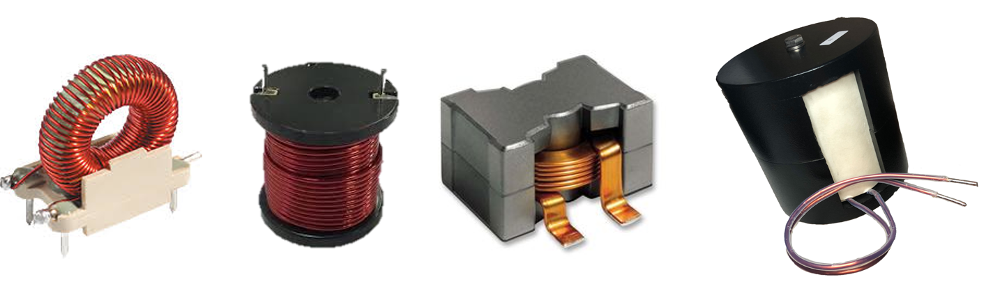
A power inductor is mainly composed of a winding and a magnetic core.
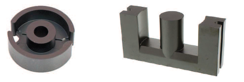
There are different types of inductances that differ in the shape and material of the ferromagnetic core. The following figure shows two forms of ferrite pots. Generally, ferromagnetic cores of inductances respect geometrical similarities. In other words, all geometric ratios are preserved when the geometric dimensions change.
10.5.2. Characteristical equations of an inductor#
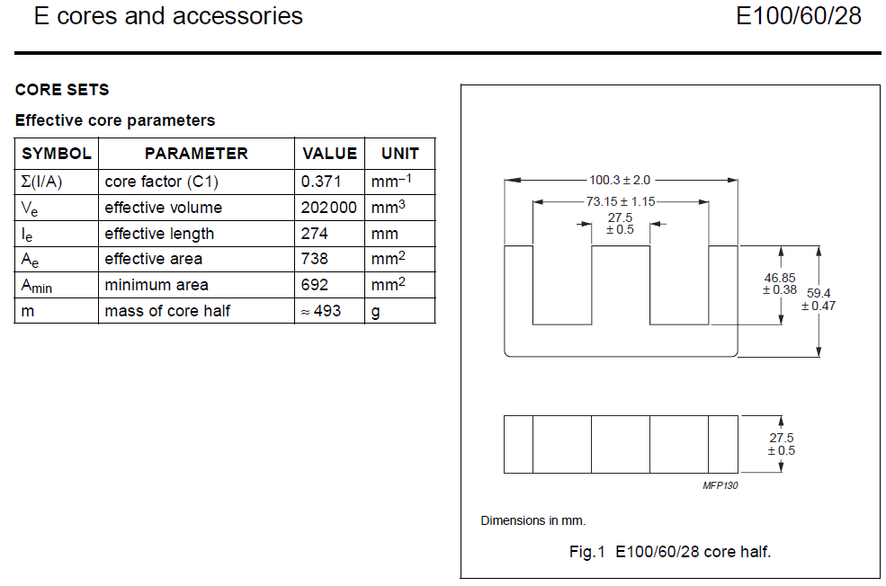
We will give here the equations allowing to calculate an inductance starting from its geometrical configuration. Here we use a ferrite pot with a E core geometry (as shown below).

An inductance \(L\) expresses the relationship between a current \(I\) and a magnetic flux \(\phi\): \(\phi=LI\)
The magnetic flux is calculated by surface integration of the magnetic field \(B\): \(\varphi= \iint\vec{B}.d\vec{S}\)
The inductance contains generally a coil of multiple turns (N turns) which see the global magnetic flux: \(\phi=N.\varphi\)
The Lenz Law express the induced voltage \(e\) in a winding of N turns: \(e=-Ndφ/dt\)
With receptor convention, the Lenz Law gives the well-known relation for an inductance (auto-induction):
\(U=LdI/dt\)
The Magnetic field \(B\) can be evaluated with the following relationships:
The conservation of the magnetic flow: \(\iint\vec{B}.d\vec{S}=0\) for a closed surface or \(\iint\vec{B_{in}}.d\vec{S}=\iint\vec{B_{out}}.d\vec{S}\)
The Ampere theorem: \(\oint \frac{\vec{B}}{\mu}.d\vec{l}=NI\) with \(\mu=\mu_0\mu_r\) the permeability of materials (\(\mu_0=4\pi10^{-7}\)).
A winding with multiple turns and the use of ferromagnetic material with high \(\mu_r\) increase the induction.
Exercice: demonstrate that the stored magnetic energy and inductance value can be expressed by the following relationships
\(\frac{1}{2}LI^2=\frac{1}{2}\frac{B^2}{\mu_0}2A_{iron}e\) and \(L=N^2\frac{\mu_0A_{iron}}{2e}\)
10.5.3. Design graph#
The equations that can be used for the inductor design are given below:

Exercice: Give the scaling laws usefull for the problem (part 5 of equations)
These equations can be represented graphically on a non oriented design graph:
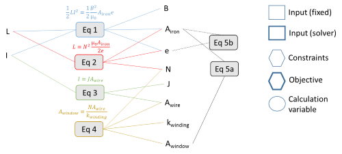
Exercice: Orientate the diagram and give the nature of each parameter (input, constraint, objective, …).
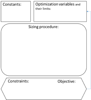
Exercice: Give now the pseudo-code wich can be used for an inductor sizing.
10.5.4. Objectives and specifications#
# Specifications
IL_max=150 # [A] max current
IL_RMS=140 # [A] RMS current
L=150e-6 # [H] Inductance

# Assumptions
J=5e6 # [A/m²] Current density
B_mag_max=0.4 # [T] Induction
k_bob=0.33 # [-] winding coefficient

# Physical constants
mu_0=4*3.14e-7 # [SI] permeability
10.5.5. Sizing code#
More details in the setting up of sizing code can be found in the following paper:
Reysset, A., Budinger, M., & Maré, J. C. (2015). Computer-aided definition of sizing procedures and optimization problems of mechatronic systems. Concurrent Engineering, 23(4), 320-332.
The sizing code is defined here in a function which can give an evaluation of the objective and an evaluation of the constraints.
We can take as reference the following E-core :
import scipy
import scipy.optimize
from math import pi, sqrt
import timeit

# Reference parameters for scaling laws (E core)

Airon_ref=738e-6    # [m^2] iron surface

A_ref=100.3e-3    # [m] E core dimension
B_ref=73.15e-3    # [m] E core dimension
C_ref=27.5e-3     # [m] E core dimension
D_ref=46.85e-3     # [m] E core dimension
E_ref=59.4e-3     # [m] E core dimension
F_ref=27.5e-3     # [m] E core dimension

M_ref=493e-3  # [kg] 1 E core mass

# -----------------------
# sizing code
# -----------------------
# inputs:
# - param: optimisation variables vector
# - arg: selection of output
# output:
# - objective if arg='Obj', problem characteristics if arg='Prt', constraints other else

def SizingCode(param, arg):
    # Variables
    e=param[0] # [m] air gap
    B_mag=param[1] # [T] induction

    # Magnetic energy calculation
    E_mag=1/2*L*IL_max**2 # [J] Energy
    A_iron= E_mag*2*mu_0/B_mag**2/2/e # [m^2] Iron surface

    # Reluctance and inductance
    Re=2*e/mu_0/A_iron  # [] reluctance
    N=sqrt(L*Re) # [-] turn number

    # Wire section & winding surface
    S_w=IL_RMS/J # [m²] 1 wire section area
    S_bob=N*S_w/k_bob # [m^2] winding surface

    # E core scaling
    A=A_ref*(A_iron/Airon_ref)**(1/2) # [m] A core dimension
    B=B_ref*(A_iron/Airon_ref)**(1/2) # [m] B core dimension
    C=C_ref*(A_iron/Airon_ref)**(1/2) # [m] C core dimension
    D=D_ref*(A_iron/Airon_ref)**(1/2) # [m] D core dimension
    E=E_ref*(A_iron/Airon_ref)**(1/2) # [m] E core dimension
    F=F_ref*(A_iron/Airon_ref)**(1/2) # [m] F core dimension

    M_core =M_ref*(A_iron/Airon_ref)**(3/2) # [kg] one E core mass

    # Core winding surface
    A_core_winding=2*D*(B-C)/2
    e_max=0.1*C

    # Mass
    M_copper=2*pi*(B+C)/4*N*S_w*7800
    M_total=M_copper+M_core*2

        # Objective and contraints
    if arg=='Obj':
        return M_total
    elif arg=='Prt':
        print("* Optimisation variables:")
        print("           Airgap e = %.2f mm"% (e*1e3))
        print("           Induction B = %.2f T"% (B_mag))
        print("* Components characteristics:")
        print("           Core (2) mass = %.2f kg" % (2*M_core))
        print("           Coil mass = %.2f kg" % M_copper)
        print("           Core dimensions = %.0f x %.0f x %.0f mmm"%((A*1e3,2*E*1e3,2*F*1e3)))
        print("           A_iron = %.0f mm^2"%(A_iron*1e6))
        print("           Number of turns = %i"%(N))
        print("* Constraints (should be >0):")
        print("           Winding  surface margin = %.3f mm²" % ((A_core_winding-S_bob)*1e6))
        print("           Airgap margin = %.3f mm" %((e_max-e)*1e3))
    else:
        return [A_core_winding-S_bob, e_max-e]
10.5.6. Optimization problem#
We will now use the opmization algorithms of the Scipy package to solve and optimize the configuration. We use here the SLQP algorithm without explicit expression of the gradient (Jacobian). A short course on Multidisplinary Gradient optimization algorithms and gradient optimization algorithm is given here:
Joaquim R. R. A. Martins (2012). A Short Course on Multidisciplinary Design Optimization. Univeristy of Michigan
The first step is to give an initial value of optimisation variables:
#Variables d'optimisation
e=10e-3 # [m] airgap
B=.2 # [T] Induction

# Vector of parameters
parameters = [e, B]
We can print of the characteristics of the problem before optimization with the intitial vector of optimization variables:
# Initial characteristics before optimization
print("-----------------------------------------------")
print("Initial characteristics before optimization :")

SizingCode(parameters, 'Prt')
print("-----------------------------------------------")
-----------------------------------------------
Initial characteristics before optimization :
* Optimisation variables:
           Airgap e = 10.00 mm
           Induction B = 0.20 T
* Components characteristics:
           Core (2) mass = 18.97 kg
           Coil mass = 1.96 kg
           Core dimensions = 269 x 318 x 147 mmm
           A_iron = 5299 mm^2
           Number of turns = 21
* Constraints (should be >0):
           Winding  surface margin = 13554.169 mm²
           Airgap margin = -2.631 mm
-----------------------------------------------
Then we can solve the problem and print of the optimized solution:
# optimization with SLSQP algorithm
contrainte=lambda x: SizingCode(x, 'Const')
objectif=lambda x: SizingCode(x, 'Obj')
result = scipy.optimize.fmin_slsqp(func=objectif, x0=parameters,
                                   bounds=[(.1e-3,10e-3), (0,B_mag_max)],
                                   f_ieqcons=contrainte, iter=100, acc=1e-4)

# Final characteristics after optimization
print("-----------------------------------------------")
print("Final characteristics after optimization :")

SizingCode(result, 'Prt')
print("-----------------------------------------------")
Optimization terminated successfully    (Exit mode 0)
            Current function value: 7.844066212970824
            Iterations: 11
            Function evaluations: 23
            Gradient evaluations: 7
-----------------------------------------------
Final characteristics after optimization :
* Optimisation variables:
           Airgap e = 5.14 mm
           Induction B = 0.40 T
* Components characteristics:
           Core (2) mass = 6.44 kg
           Coil mass = 1.41 kg
           Core dimensions = 187 x 222 x 103 mmm
           A_iron = 2578 mm^2
           Number of turns = 21
* Constraints (should be >0):
           Winding  surface margin = 5618.031 mm²
           Airgap margin = 0.000 mm
-----------------------------------------------
/opt/hostedtoolcache/Python/3.9.25/x64/lib/python3.9/site-packages/scipy/optimize/_slsqp_py.py:437: RuntimeWarning: Values in x were outside bounds during a minimize step, clipping to bounds
  fx = wrapped_fun(x)