2.1. Simulation models#
The objective of simulation models is to establish the relationships between the different components of a system and to access the variables influencing the selection of these components. The sizing scenarios at system-level can often be represented by lumped parameter models simulated with static, transient or harmonic solvers.
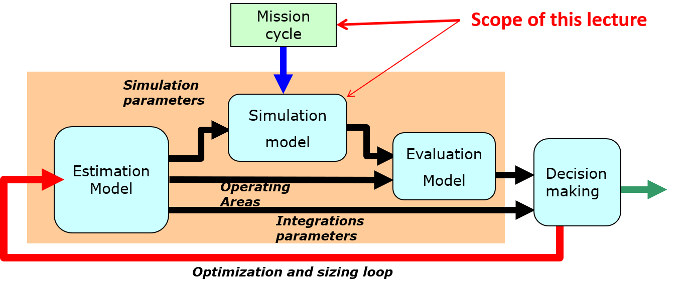
The level of modeling should be as simple as possible to minimize the number of parameters to be provided, and as fast as possible to allow optimization while giving access precisely to the design variables. Such models can be obtained by deduction or reduction methods.
For interested readers, more information can be found in the following document (Chapter 2 - Simulation models for preliminary design):
Budinger, M. (2014). Preliminary design and sizing of actuation systems (HDR dissertation, UPS Toulouse). Link
2.1.1. Differents types of scenarios and simulations#
Description
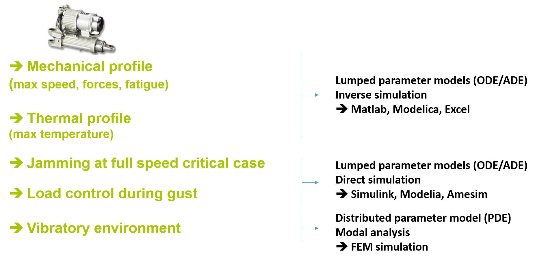
In the example of Lecture 1, the design of a spoiler actuation system requires the representation of different configurations of use called sizing scenarios. These scenarios may take the form of:
operating points with power, speed or force constants for applications with steady states.
a transient mission profile, such as a temporal mechanical profile giving access to the maximum speed, forces and fatigue of mechanical components or a transient thermal profile providing access to the thermal stress of a brushless motor;
critical events, such as jamming of the control surface, which can create violent internal efforts by the sudden deceleration of the motor inertia, or a violent gust of wind requiring a rapid decline of the control surface.
To represent the main design variables and the interaction between components, the modelling of mechatronic systems mainly uses lumped parameter models. A lumped element model simplifies the description of the behaviour of spatially distributed physical systems into a topology consisting of discrete entities.
The balance between the needs of the application and the simulation model will depend on the response times and the bandwidths to be represented:
for phenomena that vary relatively slowly, steady state or quasistatic analyses can be used. The resolution is done through a set of algebraic equations manipulating constants or harmonic amplitudes.
when the mission profiles show faster changes it may be necessary to take into account one dynamic effect, as the inertia of the rotor. This type of simulation can be represented with one state.
with rapid transients, resonance modes can be excited and add significant oscillations. This type of simulation requires several states to represent inertial and capacitive effects.
2.1.2. Typical missions profiles#
Description
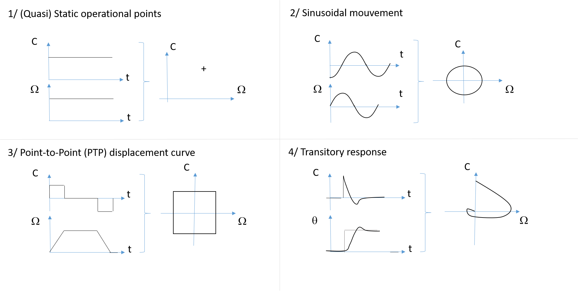
The design scenarios can take different forms:
An operational situation where power variables remains constant. This profile can be represented by an operational point in a power plot (speed,torque). These operationnal point can be used to size a device which has a constant functionning (cooling fan) or a device where interia negligeable (an hydraulics jack for instance).
sinusoidal profile they can be used to size under lifetime objectives or size an energy source.
pre-calculated transient profile.
transient response to a command reference
Operational points and mission profiles express the power demand of the load. This power requirement is often represented in a force/speed plane (or torque/speed) in order to superimpose the capacities of the actuator and the requirements of the load in the same plane.
2.1.3. Point To Point motion laws#
Description
Several applications can have a profile that describes a displacement that remains at the same value once and for all : for example the landing gear lowering, an elevator displacement,… Some shape parameters can be used to optimize the actuator on the criterion of velocity, acceleration or maximum power. Above are a few examples that concern preprogrammed displacements profils called displacement S-curves (with corresponing speed, acceleration and Jerk = acceleration derivative profiles).