Propellers estimation models with dimensional analysis and linear regressions#
Written by Marc Budinger (INSA Toulouse), Scott Delbecq (ISAE-SUPAERO) and Félix Pollet (ISAE-SUPAERO), Toulouse, France.
Propellers characteristics can be expressed by \(C_T\) and \(C_P\) coefficients. These coefficients are function of dimensions and conditions of use of propellers. Dimensional analysis and linear regression of suppliers data can be used for the generation of \(C_T\) and \(C_P\) prediction models.
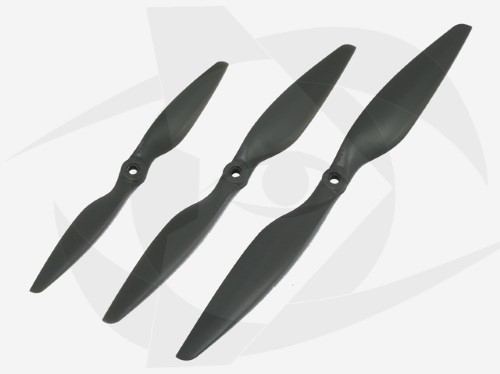
Fig. 7 APC MR (Multi-Rotor) propellers#
Dimensional analysis and \(\pi\) numbers#
The propeller performances can be expressed with 2 aerodynamic coefficients:
The thrust: \(F = C_{T} \rho_{air} n^2 D^4\)
The power: \(P = C_{P} \rho_{air} n^3 D^5 \)
The dimensional analysis and especially the Buckingham \(\pi\) theorem enable to find this results.
Dimensional analysis of the propeller thrust#
The thrust \(F\) of a propeller depends of multiple parameters (geometrical dimensions, air properties, operational points):
\(F=f(\rho_{air},n,D,p,V,\beta_{air})\)
with the parameters express in the following table.
Parameter |
M |
L |
T |
|---|---|---|---|
Thrust \(T\) [N] |
1 |
1 |
-2 |
Mass volumic (Air) \(\rho_{air}\) [kg/m\(^3\)] |
1 |
-3 |
0 |
Rotational speed \(n\) [Hz] |
0 |
0 |
-1 |
Diameter \(D\) [m] |
0 |
1 |
0 |
Pitch \(p\) [m] |
0 |
1 |
0 |
Drone speed \(V\) [m/s] |
0 |
1 |
-1 |
Bulk modulus (Air) \(\beta_{air}\) [Pa] |
1 |
-1 |
-2 |
\(=\pi_0\) |
|||
\(=\pi_1\) |
|||
\(=\pi_2\) |
|||
\(=\pi_3\) |
Remark: The dimension of a parameter \(x\) is function of dimensions L, M and T : \([x]=M^aL^bT^c\). The previous table gives the value of \(a\), \(b\) and \(c\) for each parameter of the problem.
Exercise 3
Complete the table with 4 dimensionless \(\pi\) numbers possible for the given problem. Explain the number of dimensionless number.
Solution to Exercise 3
Buckingham \(\pi\) theorem: 7 parameters - 3 dimensions = 4 dimensionless \(\pi\) numbers
Parameter |
M |
L |
T |
|---|---|---|---|
Thrust \(T\) [N] |
1 |
1 |
-2 |
Mass volumic (Air) \(\rho_{air}\) [kg/m\(^3\)] |
1 |
-3 |
0 |
Rotational speed \(n\) [Hz] |
0 |
0 |
-1 |
Diameter \(D\) [m] |
0 |
1 |
0 |
Pitch \(p\) [m] |
0 |
1 |
0 |
Drone speed \(V\) [m/s] |
0 |
1 |
-1 |
Bulk modulus (Air) \(\beta_{air}\) [Pa] |
1 |
-1 |
-2 |
\(C_t=\frac{F}{\rho n^2D^4}=\pi_0\) |
0 |
0 |
0 |
\(\frac{Pitch}{D}=\pi_1\) |
0 |
0 |
0 |
\(J=\frac{V}{nD}=\pi_2\) |
0 |
0 |
0 |
\(\frac{\rho n^2D^2}{\beta_{air}}=\pi_3\) |
0 |
0 |
0 |
Effect of the rotational speed#
APC suppliers give complete propeller data for all their propellers. From the file APC_STATIC-data-all-props.csv, we find all static data provided by APC:
import pandas as pd

# Read the .csv file with bearing data
path = "https://raw.githubusercontent.com/SizingLab/sizing_course/main/laboratories/Lab-multirotor/assets/data/"
df = pd.read_csv(path + "APC_STATIC-data-all-props.csv", sep=";")
# Print the head (first lines of the file)
df.head()
| LINE | COMP | TYPE | RPM | DIAMETER(IN) | PITCH(IN) | BLADE(nb) | THRUST(LBF) | POWER(HP) | TORQUE(IN.LBF) | Cp | Ct | AREA(m^2) | THRUST(N) | POWER(W) | ANGLE | EFF | N.D | |
|---|---|---|---|---|---|---|---|---|---|---|---|---|---|---|---|---|---|---|
| 0 | 1 | 1 | NaN | 1000 | 10.5 | 4.5 | 2 | 0.03 | 0.01 | 0.02 | 0.03 | 0.08 | 0.06 | 0.1335 | 7.457 | 0.43 | 60.180222 | 10500.0 |
| 1 | 2 | 1 | NaN | 2000 | 10.5 | 4.5 | 2 | 0.13 | 0.01 | 0.08 | 0.03 | 0.08 | 0.06 | 0.5785 | 7.457 | 0.43 | 60.180222 | 21000.0 |
| 2 | 3 | 1 | NaN | 3000 | 10.5 | 4.5 | 2 | 0.29 | 0.01 | 0.17 | 0.03 | 0.08 | 0.06 | 1.2905 | 7.457 | 0.43 | 60.180222 | 31500.0 |
| 3 | 4 | 1 | NaN | 4000 | 10.5 | 4.5 | 2 | 0.52 | 0.02 | 0.30 | 0.03 | 0.08 | 0.06 | 2.3140 | 14.914 | 0.43 | 60.180222 | 42000.0 |
| 4 | 5 | 1 | NaN | 5000 | 10.5 | 4.5 | 2 | 0.81 | 0.04 | 0.47 | 0.03 | 0.08 | 0.06 | 3.6045 | 29.828 | 0.43 | 60.180222 | 52500.0 |
For next steps, we keep only the Multi-Rotor type propellers (MR).
# Data Filtering
# Keeping only multirotor (MR) type
df_MR = df[df["TYPE"] == "MR"]
df_MR.head()
| LINE | COMP | TYPE | RPM | DIAMETER(IN) | PITCH(IN) | BLADE(nb) | THRUST(LBF) | POWER(HP) | TORQUE(IN.LBF) | Cp | Ct | AREA(m^2) | THRUST(N) | POWER(W) | ANGLE | EFF | N.D | |
|---|---|---|---|---|---|---|---|---|---|---|---|---|---|---|---|---|---|---|
| 135 | 147 | 8 | MR | 2000 | 10.0 | 4.5 | 2 | 0.14 | 0.01 | 0.09 | 0.04 | 0.11 | 0.05 | 0.6230 | 7.457 | 0.45 | 72.772802 | 20000.0 |
| 146 | 148 | 8 | MR | 3000 | 10.0 | 4.5 | 2 | 0.32 | 0.01 | 0.20 | 0.04 | 0.11 | 0.05 | 1.4240 | 7.457 | 0.45 | 72.772802 | 30000.0 |
| 147 | 149 | 8 | MR | 4000 | 10.0 | 4.5 | 2 | 0.57 | 0.02 | 0.36 | 0.04 | 0.11 | 0.05 | 2.5365 | 14.914 | 0.45 | 72.772802 | 40000.0 |
| 148 | 150 | 8 | MR | 5000 | 10.0 | 4.5 | 2 | 0.90 | 0.04 | 0.56 | 0.04 | 0.11 | 0.05 | 4.0050 | 29.828 | 0.45 | 72.772802 | 50000.0 |
| 149 | 151 | 8 | MR | 6000 | 10.0 | 4.5 | 2 | 1.29 | 0.08 | 0.79 | 0.04 | 0.11 | 0.05 | 5.7405 | 59.656 | 0.45 | 72.772802 | 60000.0 |
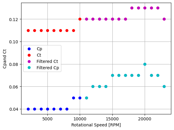
We plot the \(C_p\) and \(C_t\) for the a 10x4.5 propeller (COMP n° 8 in the previous table). We can notice that these coefficients are constant up to a certain value of speed of rotation. The manufacturer recommends using these propellers for a product speed of rotation \(\times\) diameter less than a limit (depending on the type of propeller technology) and given here:
Maximum speed(RPM) x prop diameter (inches) = 105,000
for MR type which gives a blade tip speed of 135 m/s. The dark spots on the following diagram correspond to this non-recommended operating zone.
Question: Explain the origin of this operating limit comes from and the \(\pi\) number that can express it.
Answer:
The \(\frac{\rho_{air} n^2D^2}{\beta}\) dimensionless number is similar to Mach number \(M_a=V/c\) with \(c=\sqrt{\frac{\beta_{air}}{\rho_{air}}}\) the speed of sound:
$\(\frac{\rho n^2D^2}{\beta_{air}}=M_a^2\)$
# Keep only the component n°8
df_8 = df_MR[df_MR["COMP"] == 8]

# Extract forbidden ND product
df_8_ND = df_8[df_8["N.D"] > 105000.0]

import numpy as np
import matplotlib.pyplot as plt

# Plot the data
plt.plot(df_8["RPM"], df_8["Cp"], "bo", label="Cp")
plt.plot(df_8["RPM"], df_8["Ct"], "ro", label="Ct")
plt.plot(df_8_ND["RPM"], df_8_ND["Ct"], "mo", label="Filtered Ct")
plt.plot(df_8_ND["RPM"], df_8_ND["Cp"], "co", label="Filtered Cp")
plt.xlabel("Rotational Speed [RPM]")
plt.ylabel("Cpand Ct")
plt.legend()
plt.grid()
plt.show()
Linear regression#
For next calculations, we keep only data with following criteria:
Type ‘MR’ (Multi-Rotor)
Maximum RPM < 105,000/prop diameter (inches)
# Keep only operating points with ND<105000
df_MR_ND = df_MR[df_MR["N.D"] < 105000.0]
The APC static data correspond to the hover operational point where the speed V=0. The aerodynamic coefficients are thus only a function of \(p/D\) (called ‘ANGLE’ in the .csv file) dimensionless number.
\(C_t=\frac{F}{\rho_{air} n^2 D^4}=f(\frac{p}{D})\)
\(C_p=\frac{P}{\rho_{air} n^3 D^5}=g(\frac{p}{D})\)
The following code uses the Scikit-learn package in order to set up a \(C_t\) estimator for the static case (\(V=0\) or \(J=0\)).
# Import packages
from sklearn import linear_model
from sklearn.metrics import r2_score
import matplotlib.pyplot as plt


# Data
x = df_MR_ND["ANGLE"].values
y_Ct = df_MR_ND["Ct"].values

# Matrix X and Y
X = x.reshape(-1, 1)

Y_Ct = y_Ct.reshape(-1, 1)

# Create a new object for the linear regression
reg_Ct = linear_model.LinearRegression()

reg_Ct.fit(X, Y_Ct)


# Y vector prediction
Ct_est = reg_Ct.predict(X)

# Ct Parameters
# ----
coef = float(reg_Ct.coef_)
intercept = float(reg_Ct.intercept_)
r2 = r2_score(Y_Ct, Ct_est)


# Plot the data
plt.plot(x, Y_Ct, "o", label="Reference data")
plt.plot(x, Ct_est, "-g", label="Data prediction")
plt.xlabel("Pitch/Diameter  ratio")
plt.ylabel("Ct")
plt.title("Comparison of reference data and regression")
plt.legend()
plt.grid()
plt.show()

print(f"Ct estimation model : Ct = {intercept:.2f} + {coef:.2f} * p/D with R2={r2:.3f}")
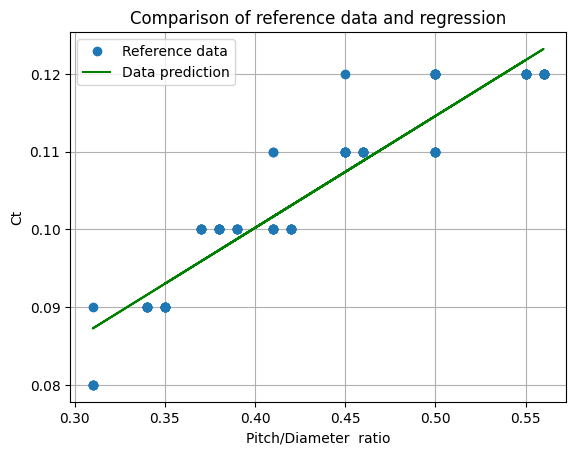
Ct estimation model : Ct = 0.04 + 0.14 * p/D with R2=0.895
Exercise 4
Perform a linear regression of \(C_p\) data.
y_Cp = df_MR_ND["Cp"].values

Y_Cp = y_Cp.reshape(-1, 1)


reg_Cp = linear_model.LinearRegression()
reg_Cp.fit(X, Y_Cp)

# Y vector prediction
Cp_est = reg_Cp.predict(X)

# Cp Parameters
# -----
coef = float(reg_Cp.coef_)
intercept = float(reg_Cp.intercept_)
r2 = r2_score(Y_Cp, Cp_est)


# Plot the data
plt.plot(x, Y_Cp, "o", label="Reference data")
plt.plot(x, Cp_est, "-g", label="Data prediction")
plt.xlabel("Pitch/Diameter  ratio")
plt.ylabel("Cp")
plt.title("Comparison of reference data and regression")
plt.legend()
plt.grid()
plt.show()

print(f"Cp estimation model : Cp = {intercept:.2f} + {coef:.2f} * p/D with R2={r2:.3f}")
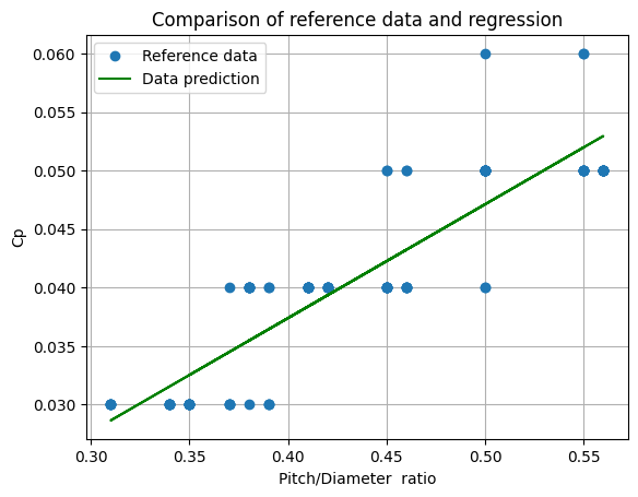
Cp estimation model : Cp = -0.00 + 0.10 * p/D with R2=0.798
Dimensional analysis of the propeller power#
The power \(P\) of a propeller depends of multiple parameters (geometrical dimensions, air properties, operational points):
\(P=f(\rho_{air},n,D,p,V,\beta_{air})\)
with the parameters express in the following table.
Parameter |
M |
L |
T |
|---|---|---|---|
Power \(P\) [W] |
1 |
2 |
-3 |
Mass volumic (Air) \(\rho_{air}\) [kg/m\(^3\)] |
1 |
-3 |
0 |
Rotational speed \(n\) [Hz] |
0 |
0 |
-1 |
Diameter \(D\) [m] |
0 |
1 |
0 |
Pitch \(p\) [m] |
0 |
1 |
0 |
Drone speed \(V\) [m/s] |
0 |
1 |
-1 |
Bulk modulus (Air) \(\beta_{air}\) [Pa] |
1 |
-1 |
-2 |
\(C_p= \frac{P}{\rho n^3 D^5} =\pi_0\) |
0 |
0 |
0 |
\(\frac{Pitch}{D}=\pi_1\) |
0 |
0 |
0 |
\(J=\frac{V}{nD}=\pi_2\) |
0 |
0 |
0 |
\(\frac{\rho n^2D^2}{\beta}=\pi_3\) |
0 |
0 |
0 |