7.7. Simulation models with Python (student version)#
Written by Marc Budinger (INSA Toulouse) and Scott Delbecq (ISAE-SUPAERO), Toulouse, France
7.7.1. Thermal model of an electric motor#
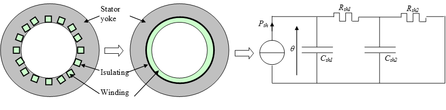
The thermal model of a motor, Figure n° 1, distinguish temperature between winding and yoke with a 2 bodies model. One can distinguish:
heat capacity of the winding: Cth1
heat capacity of the yoke: Cth2
the thermal resistance between the winding and the yoke (corresponding to the electrical insulator): Rth1
the thermal resistance between the yoke and the ambient air: Rth2
Figure n° 1 – 2 bodies thermal model of the motor
7.7.2. Modelica or state space model#
A Modelica model such as Figure 2 could be simulated in Dymola or OpenModelica.
Figure n° 2 – Modelica model
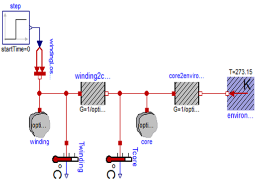
To simulate it in Python it is possible to use Functional Mock-up Units (FMU) which can be exported by system simulation softwares.
Here, we propose to use a simple state-space approach using the scipy package.
Recall: the transfert function of the problem can be expressed as
\(Z_{th}=\frac{\theta(p)}{P(p)}=R_{th,eq}\frac{1+T_0p}{1+(T_1+T_2)p+T_1T_2p}\)
with:
\(R_{th,eq}=R_1+R_2\)
\(T_0=\frac{R_1R_2}{R_1+R_2}C_2\)
\(T_1+T_2=(R_1+R_2)C_1 + R_2C_2\)
\(T_1T_2=R_1C_1R_2C_2\)
from scipy.signal import step
import numpy as np
import matplotlib.pyplot as plt
import pandas as pd


def motor_temperature(P, R1, C1, R2, C2, time=np.linspace(0, 200, 100)):
    Rtheq = R1 + R2
    T0 = R1 * R2 / (R1 + R2) * C2
    T1pT2 = (R1 + R2) * C1 + R2 * C2
    T1T2 = R1 * C1 * R2 * C2
    t, y = step(system=([Rtheq * T0, Rtheq], [T1T2, T1pT2, 1]), T=time)
    theta_winding = y * P
    d = {"t": t, "theta_winding": theta_winding}
    df = pd.DataFrame(data=d)
    return df
# Parameters
# Losses [W]
P = 100.0
# R1 [K/W]
R1 = 0.3
# C1 [J/K]
C1 = 150.0
# R2 [K/W]
R2 = 0.3
# C2 [J/K]
C2 = 150.0
# Simulation time [s]
t_final = 150.0

time = np.linspace(0, t_final, 100)

df = motor_temperature(P, R1, C1, R2, C2, time=time)
We can now access to the simulation results and plot them:
df
| t | theta_winding | |
|---|---|---|
| 0 | 0.000000 | 0.000000 |
| 1 | 1.515152 | 0.993470 |
| 2 | 3.030303 | 1.955111 |
| 3 | 4.545455 | 2.886946 |
| 4 | 6.060606 | 3.790832 |
| ... | ... | ... |
| 95 | 143.939394 | 43.250294 |
| 96 | 145.454545 | 43.464381 |
| 97 | 146.969697 | 43.675729 |
| 98 | 148.484848 | 43.884372 |
| 99 | 150.000000 | 44.090345 |
100 rows × 2 columns
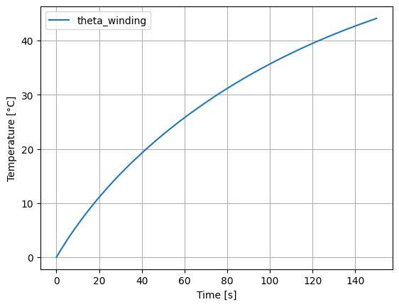
plt.plot(df["t"], df["theta_winding"])
plt.xlabel("Time [s]")
plt.ylabel("Temperature [°C]")
plt.grid()
We can access the motor final temperature:
print("Final temperature = %.2f °C" % df["theta_winding"].iloc[-1])
Final temperature = 44.09 °C
We can use interpolation to estimate intermediate temperatures:
from scipy import interpolate

theta_mot_f = interpolate.interp1d(df["t"], df["theta_winding"])

t = 100.0
theta_mot = theta_mot_f(t)

print("The temperature at t = %.2f s is %.2f °C" % (t, theta_mot))
The temperature at t = 100.00 s is 35.67 °C
7.7.3. Exercise#
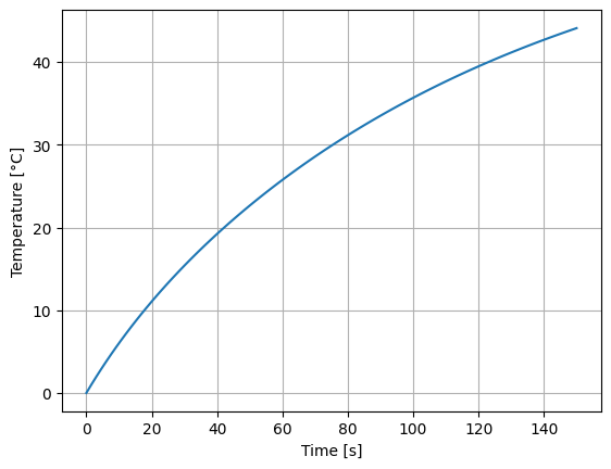
Simulate the winding temperature for 500 s and 200 W losses:
time =
P =
df =
  Cell In[7], line 1
    time =
           ^
SyntaxError: invalid syntax
plt.plot(df["t"], df["theta_winding"])
plt.xlabel("Time [s]")
plt.ylabel("Temperature [°C]")
plt.grid()
plt.legend(["theta_winding", "theta_core"], loc="upper left")
<matplotlib.legend.Legend at 0x7fbca92f4df0>