Estimation models with scaling laws and linear regression

Written by Marc Budinger (INSA Toulouse) and Scott Delbecq (ISAE-SUPAERO), Toulouse, France

The estimation models calculate the component characteristics requested for their selection without requiring a detailed design. Scaling laws are particularly suitable for this purpose. This notebook illustrates the approach with roller bearings used as thrust bearing in the linear Electro-mechanical Actuator.

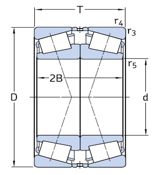
Roller bearing in face to face configuration (SKF) :

Validation of the obtained scaling laws is realized thanks linear regression on catalog data.

The following article give more details and other models for electromechanical actuators:

Budinger, M., Liscouët, J., Hospital, F., & Maré, J. C. (2012). Estimation models for the preliminary design of electromechanical actuators. Proceedings of the Institution of Mechanical Engineers, Part G: Journal of Aerospace Engineering, 226(3), 243-259.

Scaling laws

Assumptions and notation

The scaling laws use two key modelling assumptions:

1. All material properties are assumed to be identical to those of the component used for reference: \(E^* = \rho^* = ... = 1\)

2. The ratio of all the lengths of the considered component to all the lengths of the reference component is constant (geometric similarity): \(D^* = T^*= ... = d^*\)

For mechanical components, the mechanical stresses in the materials must be kept below elastic, fatigue, or contact pressure (Hertz) limits. Taking the same stress limit for a full product range yields: \( F^* = d^{*2}\)

Notation: The x* scaling ratio of a given parameter is calculated as \(x^*=\frac{x}{x_{ref}}\) where \(x_{ref}\) is the parameter taken as the reference and \(x\) the parameter under study.

Axial maximal force estimation

Propose a scaling law which links the Maximal axial force. Estimate the maximal force for a bearing of 90 mm external diameter knowing the following reference component:
\(D_{ref} = 140 mm\)
\(F_{axial,ref} = 475 kN\)

D_ref = 140  # [mm] Reference diameter
F_axial_ref = 475  # [kN] Reference max axial force

print("The estimated axial force is: %.2f kN" % (F_axial_ref * (90 / D_ref) ** 2))
print("The estimation model is: F_axial_max = %.2e.D^2" % (F_axial_ref * (1 / D_ref) ** 2))

The estimated axial force is: 196.30 kN
The estimation model is: F_axial_max = 2.42e-02.D^2

Validation with linear regression

We will validate the scaling laws obtained with regressions on catalog data.

Cleaning data

The first step is to import catalog data stored in a .csv file. We use for that functions from Panda package (with here an introduction to panda).

# Panda package Importation
import os.path as pth
import pandas as pd

# Read the .csv file with bearing data
file_path = "https://raw.githubusercontent.com/SizingLab/sizing_course/main/laboratories/Lab-vega/assets/data/bearings.csv"
df = pd.read_csv(file_path, sep=";")
# Print the head (first lines of the file)
df.head()

	d_	D	T	C	Co	Y0	Fa axial static	Pu	Wnom	Wmax	Mass
0	25	62	36.5	64.4	80	0.8	100	8.65	6000	11000	0.55
1	30	72	41.5	80.9	100	0.8	125	11.40	5300	9500	0.85
2	35	80	45.5	105.0	134	0.8	168	15.60	4500	8500	1.10
3	40	90	50.5	146.0	163	0.8	204	19.00	4500	7500	1.50
4	45	100	54.5	180.0	204	0.8	255	24.50	4000	6700	2.00

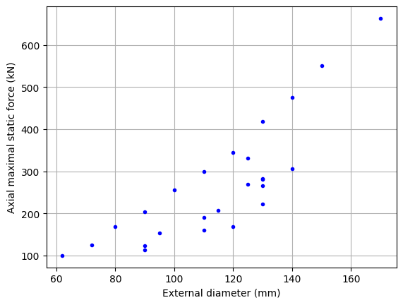
If we display these data in a scatter plot, we see that some components are not optimized in terms of axial effort.

# import plot functions from the mtplotlib package
import matplotlib.pyplot as plt

# plot
g, ax = plt.subplots(1, 1, sharex=True)
ax.plot(df["D"], df["Fa axial static"], ".b")
ax.set_ylabel("Axial maximal static force (kN)")
ax.set_xlabel("External diameter (mm)")
ax.grid()

It is interesting to clean this data in order to keep only the components representative of the problem considered. For this purpose, Pareto filtering is used where only dominant components are kept. A componant dominate another if the first is not inferior to the second in all selected objectives. Here the objective is small diameter and high maximum static force.

# This function tests if a component is dominated
# return 0 if non dominated, the number of domination other else
# inputs :
# x_,y_ : the  component's characteristics to test
# X_,Y_ : the  data set characteristics
def dominated(x_, y_, X_, Y_):
    compteur = 0
    for x, y in zip(X_, Y_):
        # x>x_ for small diameter and  y>y_ for high force
        if (x < x_) and (y > y_):
            compteur += 1
    return compteur


# We create here a new row which will give the information of component dominated or not
df["Dominated"] = False
for i in range(len(df["D"])):
    if (
        dominated(
            df.loc[i, "D"],
            df.loc[i, "Fa axial static"],
            df["D"].values,
            df["Fa axial static"].values,
        )
        > 0
    ):
        df.loc[i, "Dominated"] = True
# Print the new table
df

	d_	D	T	C	Co	Y0	Fa axial static	Pu	Wnom	Wmax	Mass	Dominated
0	25	62	36.5	64.4	80	0.8	100	8.65	6000	11000	0.55	False
1	30	72	41.5	80.9	100	0.8	125	11.40	5300	9500	0.85	False
2	35	80	45.5	105.0	134	0.8	168	15.60	4500	8500	1.10	False
3	40	90	50.5	146.0	163	0.8	204	19.00	4500	7500	1.50	False
4	45	100	54.5	180.0	204	0.8	255	24.50	4000	6700	2.00	False
5	50	90	43.5	130.0	183	1.6	114	20.80	4500	7500	1.10	True
6	50	110	58.5	208.0	240	0.8	300	28.50	3600	6000	2.60	False
7	55	90	54.0	180.0	270	2.2	123	30.50	4500	7000	1.35	True
8	55	120	63.0	209.0	275	0.8	344	33.50	3000	5600	3.30	False
9	60	95	46.0	163.0	245	1.6	153	27.00	4300	6700	1.90	True
10	60	130	67.0	246.0	335	0.8	419	40.50	2800	5300	4.10	False
11	65	120	49.5	228.0	270	1.6	169	32.50	3600	5600	1.20	True
12	65	140	72.0	281.0	380	0.8	475	47.50	2600	4800	5.05	False
13	70	110	50.0	172.0	305	1.6	191	34.50	3400	5600	1.80	True
14	70	110	62.0	220.0	400	2.5	160	45.50	3400	5600	2.40	True
15	70	150	76.0	319.0	440	0.8	550	54.00	2400	4500	6.15	False
16	75	115	62.0	233.0	455	2.2	207	52.00	3200	5300	2.40	True
17	75	125	74.0	303.0	530	1.6	331	63.00	3000	5000	3.80	True
18	75	130	54.5	238.0	355	1.6	222	41.50	3000	5000	2.85	True
19	75	130	66.5	275.0	425	1.6	266	49.00	3000	5000	3.40	True
20	80	125	58.0	233.0	430	1.6	269	49.00	3000	5000	2.65	True
21	80	140	70.5	319.0	490	1.6	306	57.00	2800	4500	4.25	True
22	80	170	85.0	380.0	530	0.8	663	64.00	2200	4000	8.75	False
23	85	130	58.0	238.0	450	1.6	281	51.00	2800	4800	2.80	True
24	85	130	72.0	308.0	620	2.2	282	69.50	2800	4800	3.55	True

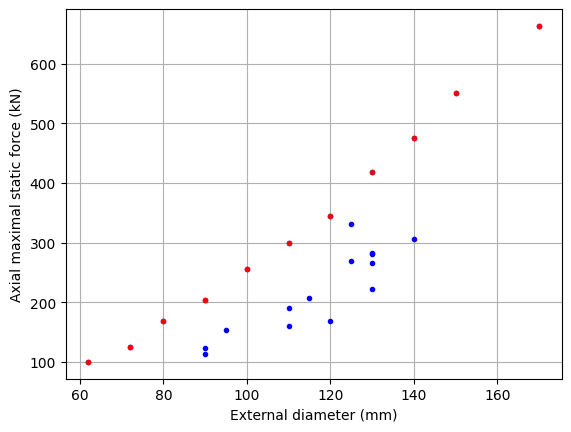
The Pareto front component are now ploted in red.

# We keep only the non dominated component (Pareto front)
df_filter = df[df["Dominated"] == False]
# Diameter of filtered bearings
df_filter_D = df_filter["D"]
# Axial force of filtered bearings
df_filter_F = df_filter["Fa axial static"]

# plot of the data set with the Pareto front
g, ax = plt.subplots(1, 1, sharex=True)
ax.plot(df["D"], df["Fa axial static"], ".b", df_filter_D, df_filter_F, ".r")
ax.set_ylabel("Axial maximal static force (kN)")
ax.set_xlabel("External diameter (mm)")
ax.grid()

Linear regression

The filtered data will be approximeted here by a linear regression of the form: \(Y=aX+b\)

We use here :

• the functions of the scikit-learn package (linear_model.LinearRegression)

• a log transformation in order to linearize the power law expression \(Y=k.X^a\) into \(log(Y) = log(k) + a.log(X)\)

A usefull introduction to machine learning can be found here Python Data Science Handbook:

VanderPlas, J. (2016). Python data science handbook: Essential tools for working with data. ” O’Reilly Media, Inc.”

with examples of linear regressions.

# Import packages
from sklearn import linear_model
import numpy as np
import matplotlib.pyplot as plt

# Create a new object for the linear regression
reg = linear_model.LinearRegression()

# Get the data :
# - X inputs and Y outputs
# - apply a log transformation in order

X = np.log10(df_filter["D"].values)

Y = np.log10(df_filter["Fa axial static"].values)

# Gives a new shape to an array without changing its data : transform data into array
X = X.reshape(-1, 1)
Y = Y.reshape(-1, 1)

# Realize the data fitting
reg.fit(X, Y)

LinearRegression()

In a Jupyter environment, please rerun this cell to show the HTML representation or trust the notebook.
On GitHub, the HTML representation is unable to render, please try loading this page with nbviewer.org.

We can now compare the coefficients of linear regression with scaling laws:

print("The coefficient are:", reg.coef_)
print("The intercept is:", reg.intercept_)
print("The estimation model is: F_axial_max = %.2e.D^%.1f" % (10**reg.intercept_, reg.coef_))

The coefficient are: [[1.91448233]]
The intercept is: [-1.43355268]
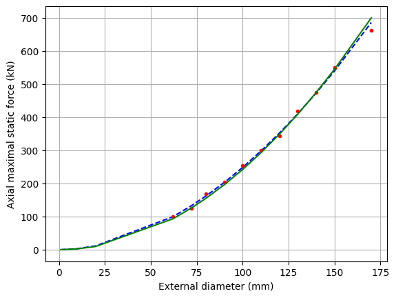
The estimation model is: F_axial_max = 3.69e-02.D^1.9

Remark : unit of \(D\) is \(mm\) and F\(_{axial,max}\) is \(kN\)

We can also directly compare on a graphic the both expressions:

# Add 1 mm diameter point
Xa = np.insert(X, 0, np.log10([1, 10, 20])).reshape(-1, 1)
# The predict function calculate the output with the regression
Yest = reg.predict(Xa)

# Scaling law
Yscal = F_axial_ref * (10**Xa / D_ref) ** 2

# plot
h, ax = plt.subplots(1, 1, sharex=True)
ax.plot(10**Xa, 10**Yest, "--b", 10**X, 10**Y, ".r", 10**Xa, Yscal, "g")
ax.set_ylabel("Axial maximal static force (kN)")
ax.set_xlabel("External diameter (mm)")
ax.grid()

10 ** reg.predict([[np.log10(90)]])

array([[203.14683888]])