
8.7. Hydrid Storage Architecture and Specification#
Written by Marc Budinger, INSA Toulouse, France
We will consider here an hybrid solutions with super capacities and traction battery packs. This notebook is dedicated :
to understand main operating limits of super capacitors and batteries
to understand a control architecture enabling to split power between super capacitors and batteries
to specify energy storage requirements of the different energy sources.
The storage element selection approach developed here is inspired by the following publication:
Jaafar, A., Sareni, B., Roboam, X., & Thiounn-Guermeur, M. (2010, September). Sizing of a hybrid locomotive based on accumulators and ultracapacitors. In 2010 IEEE Vehicle Power and Propulsion Conference (pp. 1-6). IEEE.[pdf]
8.7.1. Main operating limits of energy storage components#
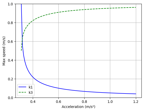
To enable the selection of energy storage means, it is necessary to understand their main operational limitations. These limits can be representative:
rapid deterioration that can develop over an operating cycle, for example one journey or a few journeys over the same day.
gradual degradation linked to the lifespan of the component over multiple cycles, months or years, where the accumulation of degradation leads to an irreversible loss of performance.
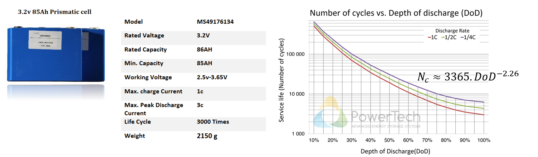
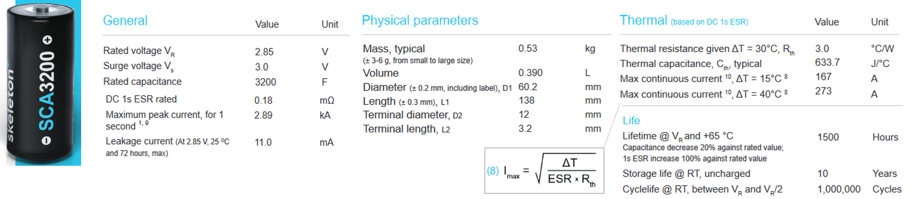
Questions: Examine the following Figures extract from datasheet of elementary storage cells of supercapacitors or battery (LiFeSO4). Propose selection criteria representative of the main operational limits. Explain how to size a battery taking into account an high number of discharge cycles.
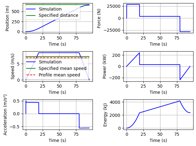
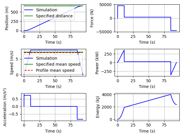
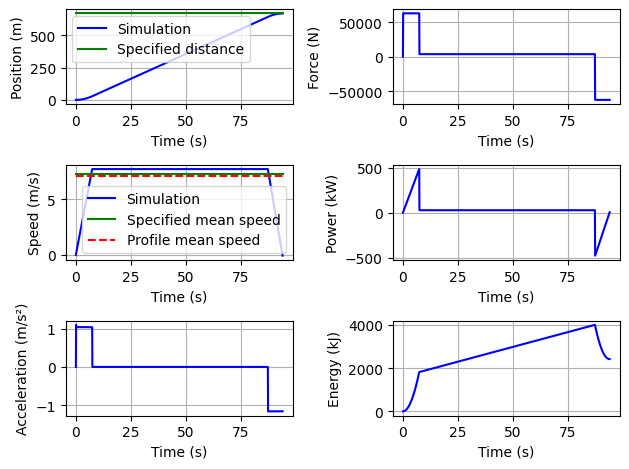
8.7.2. Simulation of a complete line#
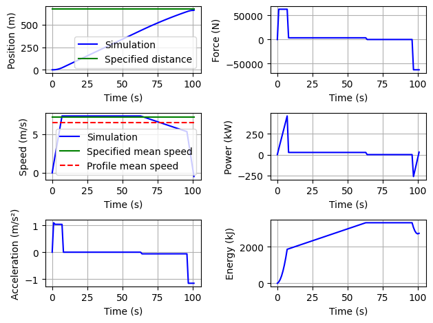
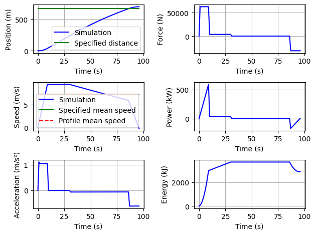
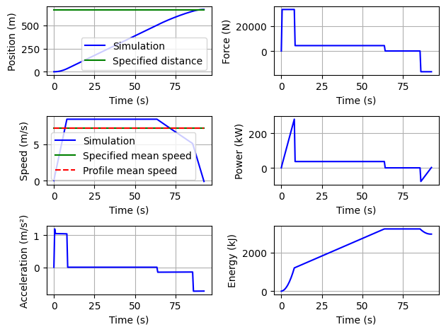
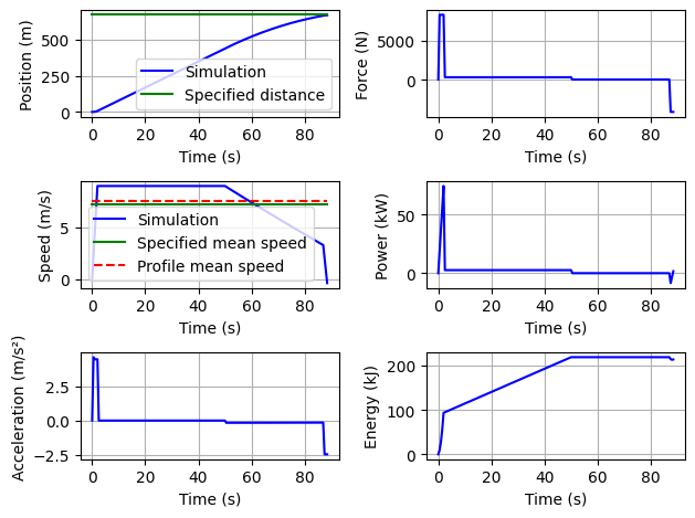
The objective of this section is to propose an evolution of the previous python codes to be able to:
simulate the power profile necessary for a complete line comprising several sections.
We will define in particular the type of vehicle, the different lengths of sections between 2 stations (Distances vector), the average speed to be ensured (Speeds vector), the presence of charger in station (Chargers vector), the stopping duration at station (StopDuration vector), the ratio between the maximum braking power and the maximum acceleration power (RatioBrakeMax).
provide the information necessary for sizing the battery/supercapacity packs that could be added.
We assume here an efficiency of the motorization chain of 100%.
Each line section will be optimized in order to meet the requirements defined previously and minimize the energy consumed. -The energy flow or the resulting power demand will be shared between battery and supercapacity with control based on frequency sharing of demands: the low frequency power will be provided by the batteries while the high frequency part will be provided by supercapacitors.
Indicators useful for sizing will then be generated from these power profiles.
take into account the energy that could come from charging stations or catenaries.
This version will only implement the consideration of charging stations.
Each charging station will provide the power to compensate for the energy of the travel from the last station.
Here we load all the functions and classes defined in the previous notebook.
%run ./01b_CaseStudy_Specification.ipynb
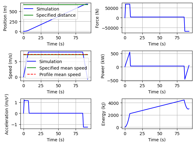
Duration of traject for given mean speed: 92.77s
Consumption per passenger: 20.44 kJ/(Pax.km)
Max energy discharge: 4450 kJ
Max power discharge: 550 kW
Max power recharge: -464 kW
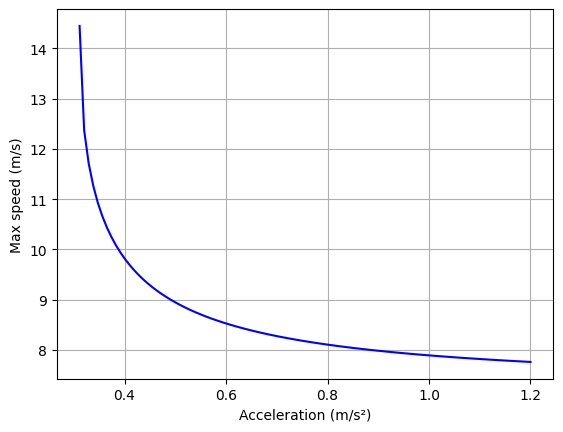
[ERROR3] Vehicle acceleration is too low , should be >0.3114059332964806m/s²

[ERROR2] Profile mean speed is too high (Vm=32.2km/h) : exceed vehicle max speed!
Max energy discharge: 4158 kJ
Max energy discharge: 4009 kJ
Max energy discharge: 3995 kJ
Positive directional derivative for linesearch    (Exit mode 8)
            Current function value: 1.2338137148050947
            Iterations: 48
            Function evaluations: 597
            Gradient evaluations: 44
Optimal vector : [0.05122318 0.667643   0.95289809]
Constraints vector : [-0.01763549366395749, -0.08872305140961852]
Consumption per passenger: 18.50 kJ/(Pax.km)
Max energy discharge: 3306 kJ
             message: Optimization terminated successfully.
             success: True
                 fun: 1.2692478005261774
                   x: [ 1.677e-01  3.027e-01  9.874e-01]
                 nit: 28
                nfev: 1309
          population: [[ 1.677e-01  3.027e-01  9.874e-01]
                       [ 1.449e-01  3.163e-01  9.899e-01]
                       ...
                       [ 1.709e-01  2.890e-01  9.746e-01]
                       [ 2.030e-01  2.624e-01  9.228e-01]]
 population_energies: [ 1.269e+00  1.270e+00 ...  1.272e+00  1.282e+00]
Optimal vector : [0.16765224 0.30271864 0.98740602]
Constraints vector : [0.02051320987779148, -0.002487562189054679]
Consumption per passenger: 19.77 kJ/(Pax.km)
Max energy discharge: 3588 kJ
             message: Optimization terminated successfully.
             success: True
                 fun: 1.2367359878503903
                   x: [ 5.747e-02  6.295e-01  9.887e-01]
                 nit: 30
                nfev: 1399
          population: [[ 5.747e-02  6.295e-01  9.887e-01]
                       [ 5.794e-02  6.378e-01  9.874e-01]
                       ...
                       [ 6.032e-02  6.234e-01  9.879e-01]
                       [ 5.727e-02  6.278e-01  9.896e-01]]
 population_energies: [ 1.237e+00  1.237e+00 ...  1.237e+00  1.237e+00]
Optimal vector : [0.05746629 0.62953101 0.98866459]
Constraints vector : [0.03335096221756688, -0.02404643449419564]
Consumption per passenger: 19.51 kJ/(Pax.km)
Max energy discharge: 3791 kJ
             message: Optimization terminated successfully.
             success: True
                 fun: 1.2218333409263697
                   x: [ 5.461e-02  7.355e-01  9.869e-01]
                 nit: 22
                nfev: 1039
          population: [[ 5.461e-02  7.355e-01  9.869e-01]
                       [ 5.418e-02  7.324e-01  9.856e-01]
                       ...
                       [ 5.505e-02  7.241e-01  9.409e-01]
                       [ 5.592e-02  7.408e-01  9.778e-01]]
 population_energies: [ 1.222e+00  1.222e+00 ...  1.230e+00  1.223e+00]
Optimal vector : [0.05461293 0.73549472 0.98690566]
Constraints vector : [0.05642389881327443, -0.0456053067993366]
Consumption per passenger: 19.70 kJ/(Pax.km)
Max energy discharge: 4031 kJ
Tramway :
             message: Optimization terminated successfully.
             success: True
                 fun: 1.2293129555100613
                   x: [ 1.557e-01  3.534e-01  9.899e-01]
                 nit: 13
                nfev: 634
          population: [[ 1.557e-01  3.534e-01  9.899e-01]
                       [ 1.147e-01  4.394e-01  9.841e-01]
                       ...
                       [ 1.406e-01  4.011e-01  9.870e-01]
                       [ 1.154e-01  4.273e-01  9.900e-01]]
 population_energies: [ 1.229e+00  1.237e+00 ...  1.236e+00  1.236e+00]
Optimal vector : [0.15565707 0.3534337  0.98986253]
Constraints vector : [0.039242456029486124, -0.03482587064676612]
Consumption per passenger: 19.55 kJ/(Pax.km)
----
Trolleybus :
             message: Optimization terminated successfully.
             success: True
                 fun: 1.083132254568939
                   x: [ 5.945e-02  7.697e-01  9.740e-01]
                 nit: 10
                nfev: 499
          population: [[ 5.945e-02  7.697e-01  9.740e-01]
                       [ 5.457e-02  9.339e-01  8.821e-01]
                       ...
                       [ 7.542e-02  7.463e-01  9.320e-01]
                       [ 5.812e-02  9.018e-01  8.547e-01]]
 population_energies: [ 1.083e+00  1.092e+00 ...  1.093e+00  1.092e+00]
Optimal vector : [0.05945318 0.76971659 0.97402578]
Constraints vector : [0.07095120144415178, 0.04063018242122724]
Consumption per passenger: 32.01 kJ/(Pax.km)
----
Bus :
             message: Optimization terminated successfully.
             success: True
                 fun: 1.1036963772929504
                   x: [ 6.029e-02  7.707e-01  9.772e-01]
                 nit: 20
                nfev: 949
          population: [[ 6.029e-02  7.707e-01  9.772e-01]
                       [ 6.008e-02  9.136e-01  8.575e-01]
                       ...
                       [ 2.072e-01  4.314e-01  9.649e-01]
                       [ 5.350e-02  8.083e-01  9.868e-01]]
 population_energies: [ 1.104e+00  1.115e+00 ...  1.146e+00  1.106e+00]
Optimal vector : [0.06028928 0.77065714 0.97719206]
Constraints vector : [0.07095120144415178, 0.04063018242122724]
Consumption per passenger: 33.54 kJ/(Pax.km)
----

Car :
             message: Optimization terminated successfully.
             success: True
                 fun: 1.208147154313186
                   x: [ 1.207e-02  6.579e-01  9.886e-01]
                 nit: 23
                nfev: 1084
          population: [[ 1.207e-02  6.579e-01  9.886e-01]
                       [ 1.096e-02  6.361e-01  9.597e-01]
                       ...
                       [ 8.411e-03  6.666e-01  9.724e-01]
                       [ 1.199e-02  7.015e-01  9.330e-01]]
 population_energies: [ 1.208e+00  1.213e+00 ...  1.224e+00  1.226e+00]
Optimal vector : [0.01206964 0.65787183 0.98859766]
Constraints vector : [-0.12028808598558105, -0.9187396351575455]
Consumption per passenger: 79.64 kJ/(Pax.km)
----
Here we define a line class with all the functionalities described just before.
from scipy import signal

class line():
    def __init__(self,Vehicle, Distances,Speeds, Chargers, StopDuration, RatioBrakeMax):
        i=0
        self.Section=[]
        self.Chargers =  Chargers # Boolean vector (True = Charger, False = No Charger , at end of te section)
        self.StopDuration = StopDuration # [s] station stop duration (scalar)
        self.RatioBrakeMax = RatioBrakeMax # [-] Ratio between max braking power / max acceleration power

        # initialization of  transient evolution (vectors)
        self.PowerStorage= [] # Transient evolution of requested power
        self.GlobalTime=[] # Time vector for plot and energy integration
        self.GlobalNRJStorage=[] # Transient evolution of energy
        self.PowerLF = [] # Transient evolution of power  (Low Frequency)
        self.PowerHF = [] # Transient evolution of power  (high Frequency)
        self.LFNRJStorage=[] # Time vector for plot and energy integration (Low Frequency)
        self.HFNRJStorage=[] # Time vector for plot and energy integration (High Frequency)

        self.TotalLineDistance =  sum(Distances)
        self.dt=0.25 # Time step for numerical integration

        # print characteristic of each section
        for d,s,c in zip(Distances,Speeds,Chargers):
            print("Section %.i: %.i m at %.2f m/s %s charger"%(i+1,d,s, "whith" if c else "without"))
            self.Section=self.Section+[OptimSection(Vehicle,d,s,self.RatioBrakeMax,self.dt)]
            i=i+1

    # Optimization loop of each section of the line
    def optimLine(self):
        X=[0.1,1,0.9]
        for i in range(len(self.Section)):
            self.Section[i].optimizeGConso(X)
            self.Section[i].plot()

    # Power vector concatenation
    def CalculPowerStorage(self):
        NRJ = 0
        self.PowerStorage= []
        self.GlobalTime= []
        dt=self.dt # [s] pas de temps pour l'integration

        # Power vector build thanks concatenation
        for i in range(len(self.Section)):
            NRJ=NRJ+self.Section[i].NRJsection[-1] # we add here the energy consummed on the section

            self.PowerStorage = self.PowerStorage + self.Section[i].psection

            # Chargers effect
            if (self.Chargers[i] == True and i<(len(self.Section)-1)):
                tcharge=NRJ/self.Section[i].Vehicle.Pmax # Charging time caculation function of energy
            else:
                tcharge=0
            if (tcharge>=self.StopDuration):
                self.PowerStorage = self.PowerStorage + [-self.Section[i].Vehicle.Pmax]*int(tcharge/dt)
                NRJ=0
            else:
                if (i<(len(self.Section)-1)):
                    self.PowerStorage = self.PowerStorage + [-self.Section[i].Vehicle.Pmax]*int(tcharge/dt)
                    self.PowerStorage = self.PowerStorage + [0]*int((self.StopDuration-tcharge)/dt)
                if (self.Chargers[i] == True) :
                    NRJ=0

        # Time vector
        t=0
        for i in range(len(self.PowerStorage)):
            self.GlobalTime = self.GlobalTime + [t]
            t = t + dt

    # Filtering of total power in order to generate LF and HF pwoers
    def FilterPower(self, omega):
        TF=signal.TransferFunction([1], [1/omega**2, 2*1/omega, 1])
        time, self.PowerLF, state = signal.lsim(TF, self.PowerStorage , self.GlobalTime)
        self.PowerHF = self.PowerStorage -  self.PowerLF

    # NRJ vector integration from power vectors
    def IntegrateNRJ(self):
        t=0
        NRJtotal=0
        NRJHF=0
        NRJLF=0
        #NRJTotalAging=0
        #NRJLFAging=0
        self.HFNRJStorage = []
        self.GlobalNRJStorage = []
        self.LFNRJStorage = []
        dt=self.dt

        for i in range(len(self.PowerStorage)):
            self.GlobalNRJStorage = self.GlobalNRJStorage + [NRJtotal]
            self.HFNRJStorage = self.HFNRJStorage + [NRJHF]
            self.LFNRJStorage = self.LFNRJStorage + [NRJLF]
            #self.TotalNRJAging = self.TotalNRJAging + [NRJTotalAging]
            #self.LFNRJAging = self.LFNRJAging + [NRJLFAging]

            t = t + dt
            NRJtotal = NRJtotal+(self.PowerStorage[i])*dt
            NRJHF = NRJHF+(self.PowerHF[i])*dt
            NRJLF = NRJLF+(self.PowerLF[i])*dt

        PmaxHF = max(abs(min(self.PowerHF)),max(self.PowerHF))/1e3 # kW
        PmaxLF = max(self.PowerLF)/1e3 # kW
        PmaxBrakeLF = abs(min(self.PowerLF))/1e3 # kW, Max power braking
        NRJHF = (max(self.HFNRJStorage) - min(self.HFNRJStorage))/3600/1e3 # NRJ en kWh
        NRJLF = (max(self.LFNRJStorage) - min(self.LFNRJStorage))/3600/1e3 # NRJ en kWh

        return PmaxHF, PmaxLF, PmaxBrakeLF, NRJHF, NRJLF


    # Main results plot
    def plot(self):

        fig, axs = plt.subplots(2,1)
        try:
            axs[0].plot(self.GlobalTime,self.PowerStorage,'b-',label='Total')
            axs[0].plot(self.GlobalTime,self.PowerLF,'r-.',label='LF')
            axs[0].plot(self.GlobalTime,self.PowerHF,'g-.',label='HF')
        except:
            pass
        axs[0].set_ylabel("Power (W)")
        axs[0].legend(bbox_to_anchor=(1.05, 1.0), loc='upper left')
        axs[0].grid()

        try:
            axs[1].plot(self.GlobalTime,self.GlobalNRJStorage,'b-',label='Total')
            axs[1].plot(self.GlobalTime,self.LFNRJStorage,'r-.',label='LF')
            axs[1].plot(self.GlobalTime,self.HFNRJStorage,'g-.',label='HF')
            axs[1].set_ylabel("Energy (J)")
            axs[1].legend(bbox_to_anchor=(1.05, 1.0), loc='upper left')
            axs[1].grid()
            axs[1].set_xlabel('Time (s)')
        except:
            fig.delaxes(axs[1])
        fig.tight_layout()
8.7.3. Example of a line definition#
We can now use this new class to define a bus transport line with the following requirements:
distances: 700, 500, 400, 700, 300, 300, 300, 300, 300, 300 m/s
mean speed: 7, 7, 7, 5, 5, 5, 5, 5 m/s
one final charger
ToulouseC=line(Bus,[700,500,400,700,300,300,300,300,300],[7, 7, 7,5,5,5,5,5],[False,False,False,False,False,False,False,True], 20, 0.6)
#ToulouseC=line(Bus,[700,500,400],[7, 7, 7],[False,False,True], 20, 0.6)
Section 1: 700 m at 7.00 m/s without charger
Section 2: 500 m at 7.00 m/s without charger
Section 3: 400 m at 7.00 m/s without charger
Section 4: 700 m at 5.00 m/s without charger
Section 5: 300 m at 5.00 m/s without charger
Section 6: 300 m at 5.00 m/s without charger
Section 7: 300 m at 5.00 m/s without charger
Section 8: 300 m at 5.00 m/s whith charger
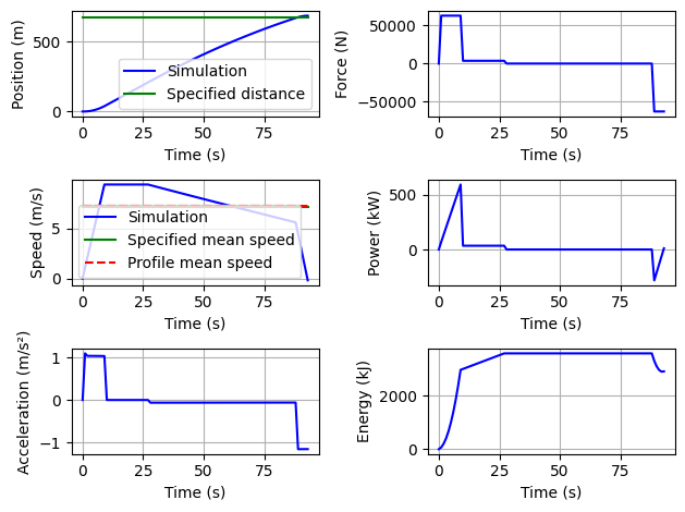
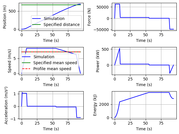
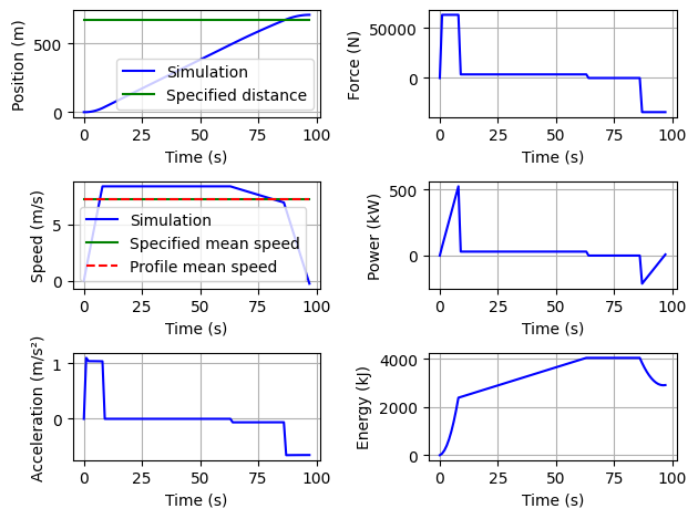
Each speed profil section can be optimized.
ToulouseC.optimLine()
---------------------------------------------------------------------------
AttributeError                            Traceback (most recent call last)
Cell In[4], line 1
----> 1 ToulouseC.optimLine()

Cell In[2], line 33, in line.optimLine(self)
     31 X=[0.1,1,0.9]
     32 for i in range(len(self.Section)):
---> 33     self.Section[i].optimizeGConso(X)
     34     self.Section[i].plot()

AttributeError: 'OptimSection' object has no attribute 'optimizeGConso'
A time vector of evolution of the power required at each section or supplied to each charger is constructed.
ToulouseC.CalculPowerStorage()
ToulouseC.plot()
---------------------------------------------------------------------------
AttributeError                            Traceback (most recent call last)
Cell In[5], line 1
----> 1 ToulouseC.CalculPowerStorage()
      2 ToulouseC.plot()

Cell In[2], line 45, in line.CalculPowerStorage(self)
     43 # Power vector build thanks concatenation
     44 for i in range(len(self.Section)):
---> 45     NRJ=NRJ+self.Section[i].NRJsection[-1] # we add here the energy consummed on the section
     47     self.PowerStorage = self.PowerStorage + self.Section[i].psection
     49     # Chargers effect

AttributeError: 'OptimSection' object has no attribute 'NRJsection'
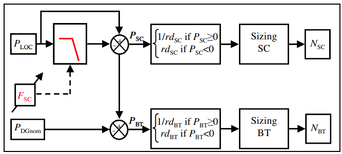
8.7.4. Hybrid storage system sizing#
The energy flow or the resulting power demand will be shared between battery and supercapacity with control based on frequency sharing of demands. The Figure below show how the low frequency power will be provided by the batteries while the high frequency part will be provided by supercapacitors.
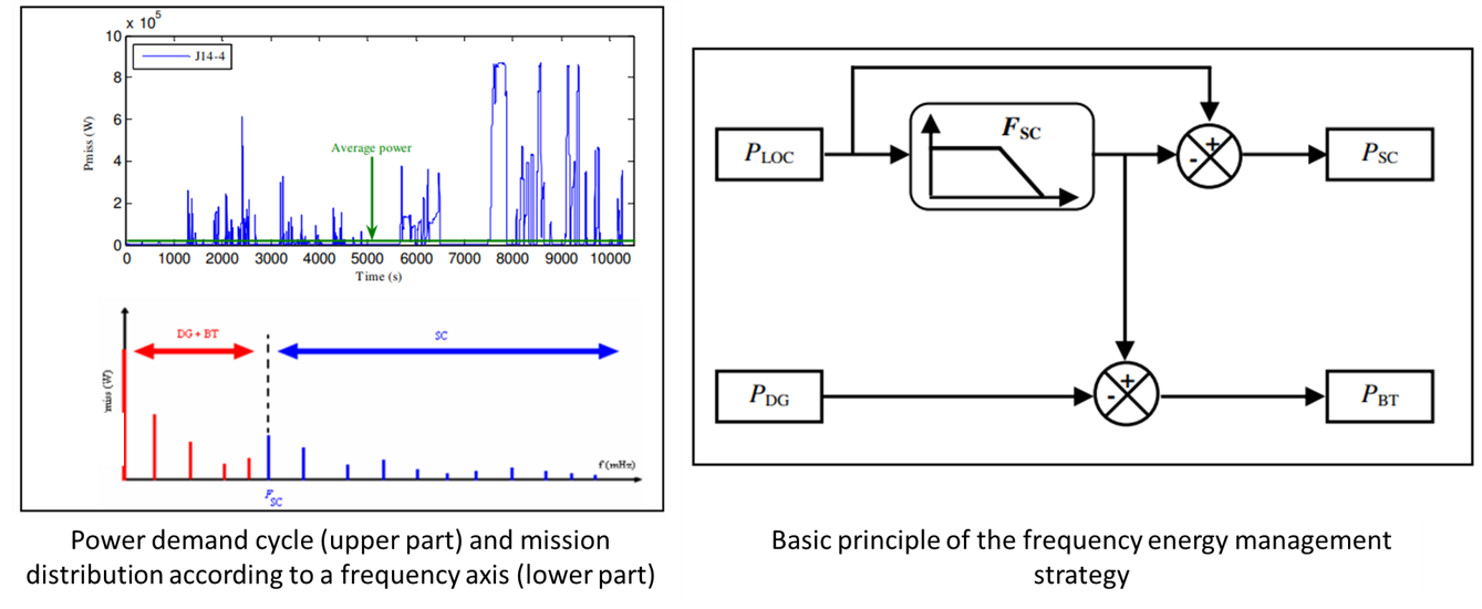
The cutoff frequency defines the power sharing and has a strong influence on the sizing of the storage elements. The following code analyzes this power sharing by varying this cutoff frequency.
Questions: Explain the sizing criteria implemented here to evaluate the mass or CO2 impact of batteries and supercapacitors.
omegaV=np.logspace(-5,2,50)
MassStorageV=[]
MassSC=[]
MassLFPAging=[]
MassLFPNRJ=[]
MassLFPPow=[]
CO2Total=[]

# Hypothese
Targetkm = 250e3 # [km] durée de vie du vehicule

# Energie massique des supercapacités
# https://1188159.fs1.hubspotusercontent-na1.net/hubfs/1188159/02-DS-220909-SKELCAP-CELLS-1F.pdf
# chez Skeleton
WmassSC=6.8*0.75 # [Wh/kg] on suppose pouvoir recuperer 75% de l'energie stockée
PmassSC=860/4.3*6.8*0.75 # [W/kg]

# Energie massique des batteries
# LFP
WmassLFP= 100 # [Wh/kg] les LFP peuvent pratiquement etre dechargé a 100%
PmassLFP=3*100 # [W/kg]  puissance massique en decharge à 3 C
PBmassLFP=1*100 # [W/kg]  puissance massique en decharge à 1 C
Ncycle = 3000 # [-] nb de cycle de decharge a 100%

# Bilan carbone
CO2SC = 39 # kgCO2eq/kg d'ecoInvent
CO2LFP = 11 # kgCO2eq/kg d'ecoInvent

for omega in omegaV:
    ToulouseC.FilterPower(omega)
    PmaxHF, PmaxLF, PmaxBrake, NRJHF, NRJLF = ToulouseC.IntegrateNRJ()

    Nc=Targetkm*1000/ToulouseC.TotalLineDistance # Number of cycles for global lifetime
    DoD=(Nc/3365)**(-1/2.26) # DoD calculation for Target Km
    MassStorageV = MassStorageV + [max(NRJHF/WmassSC*1e3, PmaxHF/PmassSC*1e3)
                                   +max(NRJLF/DoD/WmassLFP*1e3,
                                       PmaxLF/PmassLFP*1e3, PmaxBrake/PBmassLFP*1e3)]
    MassSC = MassSC + [max(NRJHF/WmassSC*1e3, PmaxHF/PmassSC*1e3)]
    MassLFPNRJ = MassLFPNRJ + [NRJLF/WmassLFP*1e3]

    MassLFPAging = MassLFPAging + [NRJLF/DoD/WmassLFP*1e3]
    MassLFPPow = MassLFPPow + [PmaxBrake/PBmassLFP*1e3]
    CO2Total = CO2Total + [max(NRJHF/WmassSC*1e3, PmaxHF/PmassSC*1e3)*CO2SC+
                           max(NRJLF/DoD/WmassLFP*1e3, PmaxLF/PmassLFP*1e3, PmaxBrake/PBmassLFP*1e3)*CO2LFP]
---------------------------------------------------------------------------
IndexError                                Traceback (most recent call last)
Cell In[6], line 30
     27 CO2LFP = 11 # kgCO2eq/kg d'ecoInvent
     29 for omega in omegaV:
---> 30     ToulouseC.FilterPower(omega)
     31     PmaxHF, PmaxLF, PmaxBrake, NRJHF, NRJLF = ToulouseC.IntegrateNRJ()
     33     Nc=Targetkm*1000/ToulouseC.TotalLineDistance # Number of cycles for global lifetime

Cell In[2], line 73, in line.FilterPower(self, omega)
     71 def FilterPower(self, omega):
     72     TF=signal.TransferFunction([1], [1/omega**2, 2*1/omega, 1])
---> 73     time, self.PowerLF, state = signal.lsim(TF, self.PowerStorage , self.GlobalTime)
     74     self.PowerHF = self.PowerStorage -  self.PowerLF

File /opt/hostedtoolcache/Python/3.9.23/x64/lib/python3.9/site-packages/scipy/signal/_ltisys.py:1890, in lsim(system, U, T, X0, interp)
   1887     X0 = zeros(n_states, sys.A.dtype)
   1888 xout = np.empty((n_steps, n_states), sys.A.dtype)
-> 1890 if T[0] == 0:
   1891     xout[0] = X0
   1892 elif T[0] > 0:
   1893     # step forward to initial time, with zero input

IndexError: index 0 is out of bounds for axis 0 with size 0
The following figures represent the overall mass of the solutions according to the power sharing achieved. A simple CO2 impact is also estimated.
plt.plot(omegaV, MassStorageV, 'g^', label='Total')
plt.plot(omegaV, MassSC, 'yx', label='SuperCap')
plt.plot(omegaV, MassLFPNRJ, 'bo', label='LFP NRJ')
plt.plot(omegaV, MassLFPPow, 'bx', label='LFP Power (Brake)')
plt.plot(omegaV, MassLFPAging, 'ro', label='LFP Aging')
plt.xscale('log')
plt.ylabel('Weight (kg)')
plt.xlabel('Cut off angular frequency (rad/s)')
plt.legend()
plt.show()
plt.plot(omegaV, CO2Total, 'g^', label='Total')
plt.xscale('log')
plt.ylabel('CO2  (kgCO2eq)')
plt.xlabel('Cut off angular frequency (rad/s)')
plt.legend()
plt.show()
---------------------------------------------------------------------------
ValueError                                Traceback (most recent call last)
Cell In[7], line 1
----> 1 plt.plot(omegaV, MassStorageV, 'g^', label='Total')
      2 plt.plot(omegaV, MassSC, 'yx', label='SuperCap')
      3 plt.plot(omegaV, MassLFPNRJ, 'bo', label='LFP NRJ')

File /opt/hostedtoolcache/Python/3.9.23/x64/lib/python3.9/site-packages/matplotlib/pyplot.py:3794, in plot(scalex, scaley, data, *args, **kwargs)
   3786 @_copy_docstring_and_deprecators(Axes.plot)
   3787 def plot(
   3788     *args: float | ArrayLike | str,
   (...)
   3792     **kwargs,
   3793 ) -> list[Line2D]:
-> 3794     return gca().plot(
   3795         *args,
   3796         scalex=scalex,
   3797         scaley=scaley,
   3798         **({"data": data} if data is not None else {}),
   3799         **kwargs,
   3800     )

File /opt/hostedtoolcache/Python/3.9.23/x64/lib/python3.9/site-packages/matplotlib/axes/_axes.py:1779, in Axes.plot(self, scalex, scaley, data, *args, **kwargs)
   1536 """
   1537 Plot y versus x as lines and/or markers.
   1538
   (...)
   1776 (``'green'``) or hex strings (``'#008000'``).
   1777 """
   1778 kwargs = cbook.normalize_kwargs(kwargs, mlines.Line2D)
-> 1779 lines = [*self._get_lines(self, *args, data=data, **kwargs)]
   1780 for line in lines:
   1781     self.add_line(line)

File /opt/hostedtoolcache/Python/3.9.23/x64/lib/python3.9/site-packages/matplotlib/axes/_base.py:296, in _process_plot_var_args.__call__(self, axes, data, *args, **kwargs)
    294     this += args[0],
    295     args = args[1:]
--> 296 yield from self._plot_args(
    297     axes, this, kwargs, ambiguous_fmt_datakey=ambiguous_fmt_datakey)

File /opt/hostedtoolcache/Python/3.9.23/x64/lib/python3.9/site-packages/matplotlib/axes/_base.py:486, in _process_plot_var_args._plot_args(self, axes, tup, kwargs, return_kwargs, ambiguous_fmt_datakey)
    483     axes.yaxis.update_units(y)
    485 if x.shape[0] != y.shape[0]:
--> 486     raise ValueError(f"x and y must have same first dimension, but "
    487                      f"have shapes {x.shape} and {y.shape}")
    488 if x.ndim > 2 or y.ndim > 2:
    489     raise ValueError(f"x and y can be no greater than 2D, but have "
    490                      f"shapes {x.shape} and {y.shape}")

ValueError: x and y must have same first dimension, but have shapes (50,) and (0,)
A Pareto front can help find a solution achieving a compromise between 2 objectives.
# Pareto Front

plt.scatter(MassStorageV, CO2Total, c=np.log10(omegaV))
plt.xlabel('Weight (kg)')
plt.ylabel('CO2  (kgCO2eq)')
plt.colorbar()
plt.title('Cut off angular frequency influence on Pareto Front')
plt.show()
---------------------------------------------------------------------------
ValueError                                Traceback (most recent call last)
File /opt/hostedtoolcache/Python/3.9.23/x64/lib/python3.9/site-packages/matplotlib/axes/_axes.py:4618, in Axes._parse_scatter_color_args(c, edgecolors, kwargs, xsize, get_next_color_func)
   4617 try:  # Is 'c' acceptable as PathCollection facecolors?
-> 4618     colors = mcolors.to_rgba_array(c)
   4619 except (TypeError, ValueError) as err:

File /opt/hostedtoolcache/Python/3.9.23/x64/lib/python3.9/site-packages/matplotlib/colors.py:512, in to_rgba_array(c, alpha)
    511 else:
--> 512     rgba = np.array([to_rgba(cc) for cc in c])
    514 if alpha is not None:

File /opt/hostedtoolcache/Python/3.9.23/x64/lib/python3.9/site-packages/matplotlib/colors.py:512, in <listcomp>(.0)
    511 else:
--> 512     rgba = np.array([to_rgba(cc) for cc in c])
    514 if alpha is not None:

File /opt/hostedtoolcache/Python/3.9.23/x64/lib/python3.9/site-packages/matplotlib/colors.py:314, in to_rgba(c, alpha)
    313 if rgba is None:  # Suppress exception chaining of cache lookup failure.
--> 314     rgba = _to_rgba_no_colorcycle(c, alpha)
    315     try:

File /opt/hostedtoolcache/Python/3.9.23/x64/lib/python3.9/site-packages/matplotlib/colors.py:398, in _to_rgba_no_colorcycle(c, alpha)
    397 if not np.iterable(c):
--> 398     raise ValueError(f"Invalid RGBA argument: {orig_c!r}")
    399 if len(c) not in [3, 4]:

ValueError: Invalid RGBA argument: -5.0

The above exception was the direct cause of the following exception:

ValueError                                Traceback (most recent call last)
Cell In[8], line 3
      1 # Pareto Front
----> 3 plt.scatter(MassStorageV, CO2Total, c=np.log10(omegaV))
      4 plt.xlabel('Weight (kg)')
      5 plt.ylabel('CO2  (kgCO2eq)')

File /opt/hostedtoolcache/Python/3.9.23/x64/lib/python3.9/site-packages/matplotlib/pyplot.py:3903, in scatter(x, y, s, c, marker, cmap, norm, vmin, vmax, alpha, linewidths, edgecolors, plotnonfinite, data, **kwargs)
   3884 @_copy_docstring_and_deprecators(Axes.scatter)
   3885 def scatter(
   3886     x: float | ArrayLike,
   (...)
   3901     **kwargs,
   3902 ) -> PathCollection:
-> 3903     __ret = gca().scatter(
   3904         x,
   3905         y,
   3906         s=s,
   3907         c=c,
   3908         marker=marker,
   3909         cmap=cmap,
   3910         norm=norm,
   3911         vmin=vmin,
   3912         vmax=vmax,
   3913         alpha=alpha,
   3914         linewidths=linewidths,
   3915         edgecolors=edgecolors,
   3916         plotnonfinite=plotnonfinite,
   3917         **({"data": data} if data is not None else {}),
   3918         **kwargs,
   3919     )
   3920     sci(__ret)
   3921     return __ret

File /opt/hostedtoolcache/Python/3.9.23/x64/lib/python3.9/site-packages/matplotlib/__init__.py:1473, in _preprocess_data.<locals>.inner(ax, data, *args, **kwargs)
   1470 @functools.wraps(func)
   1471 def inner(ax, *args, data=None, **kwargs):
   1472     if data is None:
-> 1473         return func(
   1474             ax,
   1475             *map(sanitize_sequence, args),
   1476             **{k: sanitize_sequence(v) for k, v in kwargs.items()})
   1478     bound = new_sig.bind(ax, *args, **kwargs)
   1479     auto_label = (bound.arguments.get(label_namer)
   1480                   or bound.kwargs.get(label_namer))

File /opt/hostedtoolcache/Python/3.9.23/x64/lib/python3.9/site-packages/matplotlib/axes/_axes.py:4805, in Axes.scatter(self, x, y, s, c, marker, cmap, norm, vmin, vmax, alpha, linewidths, edgecolors, plotnonfinite, **kwargs)
   4802 if edgecolors is None:
   4803     orig_edgecolor = kwargs.get('edgecolor', None)
   4804 c, colors, edgecolors = \
-> 4805     self._parse_scatter_color_args(
   4806         c, edgecolors, kwargs, x.size,
   4807         get_next_color_func=self._get_patches_for_fill.get_next_color)
   4809 if plotnonfinite and colors is None:
   4810     c = np.ma.masked_invalid(c)

File /opt/hostedtoolcache/Python/3.9.23/x64/lib/python3.9/site-packages/matplotlib/axes/_axes.py:4624, in Axes._parse_scatter_color_args(c, edgecolors, kwargs, xsize, get_next_color_func)
   4622 else:
   4623     if not valid_shape:
-> 4624         raise invalid_shape_exception(c.size, xsize) from err
   4625     # Both the mapping *and* the RGBA conversion failed: pretty
   4626     # severe failure => one may appreciate a verbose feedback.
   4627     raise ValueError(
   4628         f"'c' argument must be a color, a sequence of colors, "
   4629         f"or a sequence of numbers, not {c!r}") from err

ValueError: 'c' argument has 50 elements, which is inconsistent with 'x' and 'y' with size 0.
ToulouseC.FilterPower(0.4)
PmaxHF, PmaxLF, PmaxBrakeLF, NRJHF, NRJLF=ToulouseC.IntegrateNRJ()

Nc=Targetkm*1000/ToulouseC.TotalLineDistance # Number of cycles for global lifetime
DoD=(Nc/3365)**(-1/2.26) # DoD calculation for Target Km

print("Super Capacitor:")
print("Pmax: %.2f kW"%PmaxHF)
print("NRJ:  %.2f kWh"%NRJHF)
print("Mass: % .1f kg"%(max(NRJHF/WmassSC*1e3, PmaxHF/PmassSC*1e3)))

print("---")
print("Traction battery:")
print("Pmax discharge: %.2f kW"%PmaxLF)
print("Pmax charge: %.2f kW"%PmaxBrakeLF)
print("NRJ: %.2f kWh"%(NRJLF/DoD))
print("NRJ one travel: %.2f kWh"%(NRJLF))
print("Mass: % .1f kg"%(max(NRJLF/DoD/WmassLFP*1e3,
                                       PmaxLF/PmassLFP*1e3, PmaxBrakeLF/PBmassLFP*1e3)))
print("Mass (brake criteria): % .1f kg"%(PmaxLF/PmassLFP*1e3))


ToulouseC.plot()
print("---")
---------------------------------------------------------------------------
IndexError                                Traceback (most recent call last)
Cell In[9], line 1
----> 1 ToulouseC.FilterPower(0.4)
      2 PmaxHF, PmaxLF, PmaxBrakeLF, NRJHF, NRJLF=ToulouseC.IntegrateNRJ()
      4 Nc=Targetkm*1000/ToulouseC.TotalLineDistance # Number of cycles for global lifetime

Cell In[2], line 73, in line.FilterPower(self, omega)
     71 def FilterPower(self, omega):
     72     TF=signal.TransferFunction([1], [1/omega**2, 2*1/omega, 1])
---> 73     time, self.PowerLF, state = signal.lsim(TF, self.PowerStorage , self.GlobalTime)
     74     self.PowerHF = self.PowerStorage -  self.PowerLF

File /opt/hostedtoolcache/Python/3.9.23/x64/lib/python3.9/site-packages/scipy/signal/_ltisys.py:1890, in lsim(system, U, T, X0, interp)
   1887     X0 = zeros(n_states, sys.A.dtype)
   1888 xout = np.empty((n_steps, n_states), sys.A.dtype)
-> 1890 if T[0] == 0:
   1891     xout[0] = X0
   1892 elif T[0] > 0:
   1893     # step forward to initial time, with zero input

IndexError: index 0 is out of bounds for axis 0 with size 0
8.7.5. Labwork and homework#
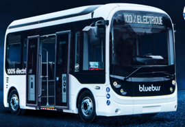
Your objective is to specify the hybrid storage system of an electric bus for doubling line 78 between the IUT Rangueil and MFJA stations.
The characteristics of the bus are here
 A example of time table of the line 78 is here
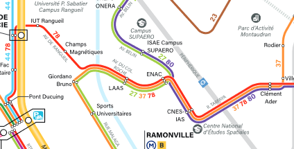 We will assume a round trip in 20 min, charge at the ends of the lines included.
Modify the present notebooks in order to set up a technical justification report : starting from the need (journey, vehicle size, frequency of journeys), setting up the effort/speed/power profiles, the power distribution in the hybrid storage system, the preliminary sizing and the specification of the main components.
Adapt and complete the sizing process in order to take into account the global efficiency of the converters and storage elments (assumed to be equal to 80%).
Propose compatible technological storage packs and specify the DC/DC converters (DC bus of 400 V).
Provide an electrical architecture diagram (possible software) summarizing your main choices:
representing the different sources and load of the network.
making it possible to standardize the DC/DC converters used.
allowing reduced functionality to be maintained in the event of a fault on part of the storage elements