7.3. Modeling of the mechanical load#
Written by Marc Budinger (INSA Toulouse) and Scott Delbecq (ISAE-SUPAERO), Toulouse, France
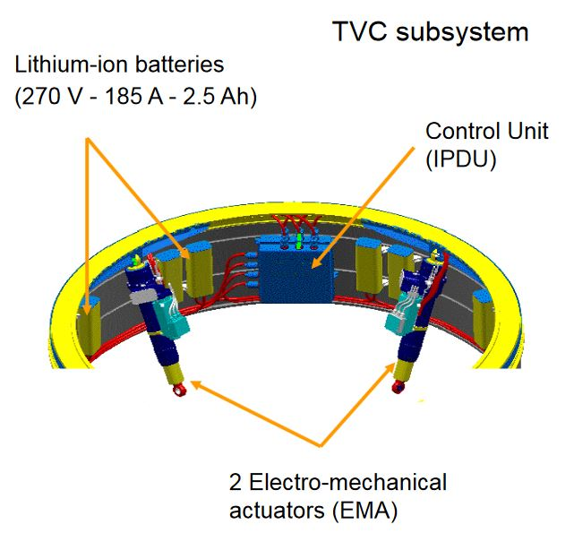
The actuation system of the 1st stage of the launcher consists of a set of Lithium-ion batteries, a control unit (2 inverters and control/command electronics) and two electromechanical actuators (EMA). This set makes it possible to control the nozzle according to 2 axes of rotation. We will be interested here only in one axis axis of rotation and we will neglect the couplings between these 2 axes.
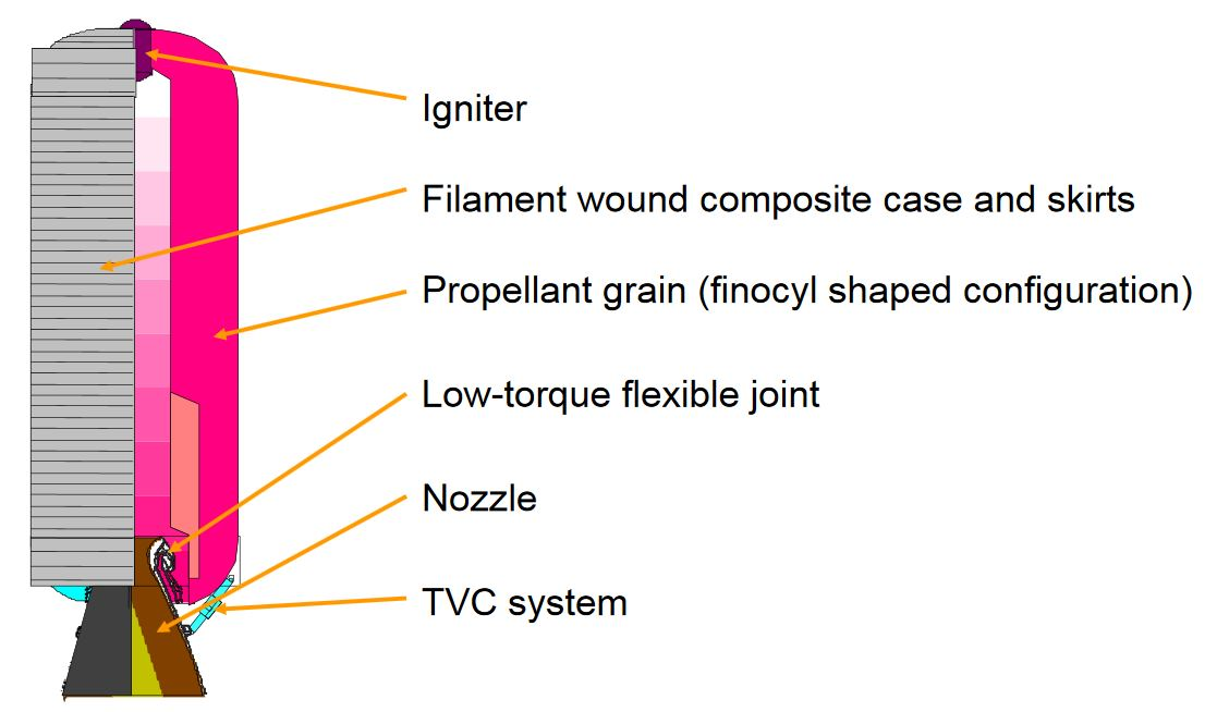
Vega Launcher 1st stage (P80) :

Thrust Vector Control (TVC) actuation system :

7.3.1. Nozzle modeling#
from IPython.display import Markdown as md  # enable Markdown printing

# Definition of nozzle equivalent parameters with engineering units
Jnozzle = 1.40e03  # [kg.m2] Inertia
Knozzle = 1.52e04  # [Nm/deg] Stiffness
Fnozzle = 1.74e02  # [Nms/deg] Viscous damping

#
md(
    """
The nozzle is composed of :
- a flexible bearing or flexseal which links the nozzle to the launcher and enables rotational movement. The equivalent characteristics and parameters for this flexible bearing are:
    - a **stiffness** of {:.0f} Nm/deg.
    - a **viscous damping** of {:.0f}	Nms/deg
- a rigid cone modeled here as:
    - an **inertia** of {:.0f} kg.m^2
    """.format(
        Knozzle, Fnozzle, Jnozzle
    )
)
The nozzle is composed of :
a flexible bearing or flexseal which links the nozzle to the launcher and enables rotational movement. The equivalent characteristics and parameters for this flexible bearing are:
a stiffness of 15200 Nm/deg.
a viscous damping of 174 Nms/deg
a rigid cone modeled here as:
an inertia of 1400 kg.m^2
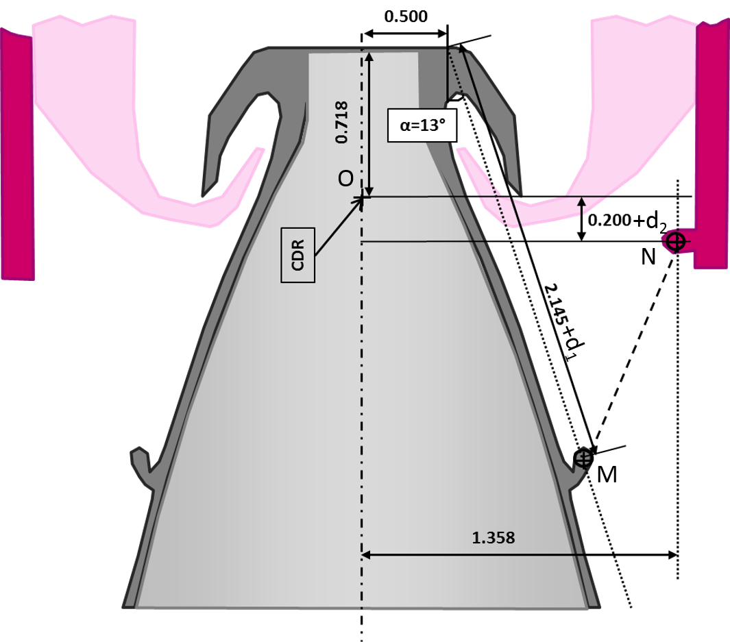
P80 Nozzle (from [ESA presentation]
(http://www.ingaero.uniroma1.it/attachments/1609_VEGA sapienza small.pdf)):

# import math package whic contains usefull mathematical functions and variables
import math
import numpy as np

# Calculate SI unit values of Knozzle and Fnozzle
# pi value is math.pi

# student part -------------
Knozzle = Knozzle / (math.pi / 180)
Fnozzle = Fnozzle / (math.pi / 180)
# --------------------------

# Print the corresponding values with print("xxx %f xxx %f "%(value1,value2)
md(
    """
>Remark: SI unit conversion of these parameters *K<sub>nozzle</sub>* = {:.2e} Nm/rad and *F<sub>nozzle</sub>* = {:.2e} Nms/rad
""".format(
        Knozzle, Fnozzle
    )
)
Remark: SI unit conversion of these parameters Knozzle = 8.71e+05 Nm/rad and Fnozzle = 9.97e+03 Nms/rad
7.3.1.1. Lever arm calculation#
The EMA (Electro Mechanical Actuator) is between M and N points of the following drawing. The given values correspond to a nominal case. But during the sizng we want to evaluate and optimize the position of N and M points. d1 and d2 are thus design variables.
P80 Nozzle section :

For the following steps, we need to calculate the equivalent lever arm between the linear displacement of the actuator and the rotational displacement of the nozzle. Thanks to the Sympy package, a symbolic calculation of this lever arm, function of d1 and d2, is possible.
Remember that the link between the torque T on the nozzle and the force F of the actuator can be calculated with the following cross product:
\(\vec{T}=\vec{OM} \times \vec{F}=\vec{OM} \times \frac{\vec{NM}}{\left|\vec{NM}\right|} F \)
thus the equivalent lever arm can be calculated with:
\(L_{arm}=\left| \vec{OM} \times \frac{\vec{NM}}{\left|\vec{NM}\right|} \right|\)
and the torque can be calculated with the simple equation:
\(T=L_{arm}.F\)
Remark: the variation of lever arm with position order is assumed to be negligeable here due to the small nozzle deflection (+/- 5.7° max)
# import vector manipulation and symbols definition of Sympy
from sympy.physics.mechanics import ReferenceFrame, Vector
from sympy import symbols, lambdify
import sympy

alpha = 13 * 3.14 / 180  # [rad] cone angle

# definition of d1 and d2 variable for symbolic calculation
d1, d2 = symbols("d1 d2")

# definition of a reference frame for vectors definiions
N = ReferenceFrame("N")

# definition of OM and ON vectors thanks N.x and N.y reference (unit) vectors
OM = (0.5 + (2.145 + d1) * np.sin(alpha)) * N.x + (0.718 - (2.145 + d1) * np.cos(alpha)) * N.y

ON = 1.358 * N.x - (0.2 + d2) * N.y

# Actuator length
NM = OM - ON

# The lever arm
Larm = (OM ^ NM.normalize()).magnitude()
The expression of the actuator length is :
NM.evalf(4)
The expression of the equivalent lever arm is :
Larm.evalf(4)
This expression can be evaluated:
at the nominal anchorage point (d1=0 and d2=0)
for different anchorage points
# Transform the expression into a numerical function
Evaluate_Larm = lambdify((d1, d2), Larm)

md("The lever arm for the nominal dimensions is %4.2f m" % Evaluate_Larm(0, 0))
The lever arm for the nominal dimensions is 1.35 m
# Import plot3d function  from sympy package
from sympy.plotting import plot3d

%matplotlib inline

# plot the Lever arm in function of d1 and d2 variables
plot3d(Larm, (d1, -0.1, +0.1), (d2, -0.1, +0.1), xlabel="d1", ylabel="d2", title="Lever arm")

# plot the Actuator Length in function of d1 and d2 variables
plot3d(
    NM.magnitude(),
    (d1, -0.1, +0.1),
    (d2, -0.1, +0.1),
    xlabel="d1",
    ylabel="d2",
    title="Actuator length",
)


<sympy.plotting.backends.matplotlibbackend.matplotlib.MatplotlibBackend at 0x7f517caf6a60>
7.3.2. Sizing scenarios modeling#
2 use cases must be checked during the design:
a static deflection of 5.7 °
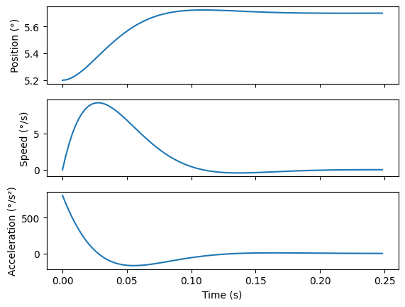
a dynamic mission profile which must ensure a response time of 72 ms for a position step from 5.2 to 5.7°.
7.3.2.1. Static sizing scenario#
The maximal angular displacement is 5.7°. The corresping force can be calculated thanks the flexible bearing stiffness.
teta_max = 5.7 * math.pi / 180

Fstat_max = Knozzle * teta_max / Evaluate_Larm(0, 0)

md("The maximum static force is %4.2e N." % Fstat_max)
The maximum static force is 6.40e+04 N.
7.3.2.2. Dynamic sizing scenario#
For this scenario, we will assume that the position close loop system will response as a second order filter between real position and order:
\(H(p)=\frac{1}{1+\frac{2\xi p}{\omega_0}+\frac{p^2}{\omega_0^2}}\)
with \(\xi=0.7\) and thus \(t_{r5}=\frac{2.9}{\omega_0}\)
We calculate here position, speed and acceleration of the nozzle for a step request (5.2 to 5.7° in 72 ms).
# Import from scipy of the step response
from scipy.signal import step

# Definition of time response, damping coef, and angular frequency of the filter
tr = 72e-3
w0 = 2.9 / tr
eps = 0.7

# position calculation with a second order step response
num = [1.0]
den = [1 / w0**2, 2 * eps / w0, 1]
t, y = step(system=(num, den))
y = 5.2 + 0.5 * y

# speed, we change here only the numerator of the transfer function
nump = [1.0, 0.0]
t, yp = step(system=(nump, den))
yp = 0.5 * yp

# acceleration
nump = [1.0, 0.0, 0.0]
t, ypp = step(system=(nump, den))
ypp = 0.5 * ypp

# plot of the different dynamic answers
import matplotlib.pyplot as plt

f, (ax1, ax2, ax3) = plt.subplots(3, 1, sharex=True)
ax1.plot(t, y)
ax1.set_ylabel("Position (°)")
ax2.plot(t, yp)
ax2.set_ylabel("Speed (°/s)")
ax3.plot(t, ypp)
ax3.set_ylabel("Acceleration (°/s²)")
ax3.set_xlabel("Time (s)")
plt.show()

It’s now possible to calculate the force of the actuator which is requested to respect this mission profile.
# degree to rad
teta, tetap, tetapp = math.pi / 180 * y, math.pi / 180 * yp, math.pi / 180 * ypp

# Force calculation
Fdyn = (Jnozzle * tetapp + Fnozzle * tetap + Knozzle * teta) / Evaluate_Larm(0, 0)

g, gx1 = plt.subplots(1, 1, sharex=True)
gx1.plot(t, Fdyn)
gx1.set_ylabel("Force (N)")
gx1.set_xlabel("Time (s)")
gx1.grid()
plt.show()

7.4. Force speed diagram#
This sizing scenarios can be represented on a force-speed diagram usefull for compenent selection.
# we create here a force-speed diagram
h, hx1 = plt.subplots(1, 1, sharex=True)
hx1.plot(yp, Fdyn, "b", 0, Fstat_max, ".k")
hx1.set_ylabel("Force (N)")
hx1.set_xlabel("Speed (°/s)")
hx1.grid()
plt.show()

7.4.1. Summary#
For the next sizing steps, we will use
the nozzle max speed (step response)
the max static torque (max deflexion)
for max dynamic point (step response) : Max force with acceleration
In the nozzle frame (rotational movement):
import pandas as pd

df_rot = pd.DataFrame(
    {
        "Value": [max(yp), Knozzle * teta_max, max(Fdyn), max(ypp)],
        "Unit": ["°/s", "N.m", "N.m", "°/s²"],
    },
    index=[
        "Max nozzle rotational speed",
        "Max static torque",
        "Max dynamic torque",
        "Max acceleration",
    ],
)

pd.options.display.float_format = "{:,.2e}".format

md(df_rot.to_markdown())
| | Value | Unit | |:—————————-|————:|:——-| | Max nozzle rotational speed | 9.23502 | °/s | | Max static torque | 86640 | N.m | | Max dynamic torque | 73000.8 | N.m | | Max acceleration | 811.15 | °/s² |
For the linear actuator (translational movement) with \(d_1=0\) and \(d_2=0\):
df_lin = pd.DataFrame(
    {
        "Value": [
            Evaluate_Larm(0, 0),
            max(yp) * np.pi / 180 * Evaluate_Larm(0, 0),
            Knozzle * teta_max / Evaluate_Larm(0, 0),
            max(Fdyn),
            max(ypp) * Evaluate_Larm(0, 0) * np.pi / 180,
        ],
        "Unit": ["m", "m/s", "N", "N", "m/s²"],
    },
    index=[
        "Lever arm",
        "Max linear speed",
        "Max static force",
        "Max dynamic force",
        "Max acceleration",
    ],
)

md(df_lin.to_markdown())
| | Value | Unit | |:——————|————-:|:——-| | Lever arm | 1.35423 | m | | Max linear speed | 0.218277 | m/s | | Max static force | 63977.1 | N | | Max dynamic force | 73000.8 | N | | Max acceleration | 19.1722 | m/s² |


